

In the previous two articles we defined what a set is and how to operate on it. Now we reach a natural question: how many elements does a set have? This simple question hides an important subtlety: when two sets overlap and we want to count their union, a plain \(n(A) + n(B)\) counts some elements twice. The Inclusion-Exclusion Principle fixes this and is the first combinatorial result of this series.
Cardinality #
The cardinality of a set \(A\), denoted \(n(A)\) or \(|A|\), is the number of elements of \(A\).
This article uses \(n(A)\) to avoid ambiguity with the absolute value \(|x|\), which appears in the examples below. In the Computer Science literature, however, the notation \(|A|\) is the most common: you will find it in algorithm analysis (\(O(|V| + |E|)\) for graphs, for example) and in university-level texts on combinatorics and set theory.
We say a set is finite when its cardinality is a nonnegative integer (\(0, 1, 2, \ldots\)). Saying “natural number” would not be enough: in this series, as we saw in the first article, \(0 \notin \mathbb{N}\), and the empty set, whose cardinality is 0, would be left out. When the enumeration does not end, the set is infinite (like \(\mathbb{N}\), \(\mathbb{Z}\), \(\mathbb{R}\)).
Examples
- \(A = \{x \in \mathbb{Z} \mid |x| \leq 3\} = \{-3,-2,-1,0,1,2,3\}\) → \(n(A) = 7\)
- \(B = \{x \in \mathbb{N} \mid x \text{ is even}\} = \{2,4,6,\ldots\}\) → infinite
- \(\emptyset\) → \(n(\emptyset) = 0\)
And what about infinite sets: do they all have the same size? The question seems meaningless, but answering it is what led Georg Cantor to create set theory.
To compare sets without counting them, Cantor used bijections: two sets have the same cardinality when it is possible to pair their elements one to one, with no one left over on either side. For finite sets, this is the same as having the same number of elements; for infinite ones, it is the definition that works.
- \(\mathbb{Z}\) has the same size as \(\mathbb{N}\), even though it seems to have “twice as many” elements. Just list the integers alternating signs: \(1 \mapsto 0\), \(2 \mapsto 1\), \(3 \mapsto -1\), \(4 \mapsto 2\), \(5 \mapsto -2\), and so on. Every integer appears exactly once in the list.
- \(\mathbb{Q}\) also has the same size as \(\mathbb{N}\): the fractions \(p/q\) can be laid out in an infinite table and traversed diagonally, skipping the repeated ones (\(2/4\) has already appeared as \(1/2\)).
- \(\mathbb{R}\) is larger. By the diagonal argument (Cantor, 1891, originally formulated for infinite binary sequences and adapted here to decimals), any list of real numbers leaves some number out: just build a number whose first decimal digit differs from that of the first number in the list, the second from that of the second, and so on, using only digits other than 0 and 9 to avoid repeating decimals such as \(0.4999\ldots = 0.5\).
Infinite sets with the cardinality of \(\mathbb{N}\) are called countable, and this cardinality has a name: \(\aleph_0\) (aleph-null). Thus, \(n(\mathbb{N}) = n(\mathbb{Z}) = n(\mathbb{Q}) = \aleph_0\), while \(n(\mathbb{R}) > \aleph_0\). More at Cardinality, Countable set, and Aleph number.
These ideas of Georg Cantor (1845 to 1918) were received with hostility by some of the mathematicians of the time. Leopold Kronecker, who only accepted objects built in a finite number of steps from the natural numbers, went as far as calling him a “scientific charlatan” and a “corrupter of youth.” Cantor had his first episode of depression in 1884, went through several hospitalizations, and died in a sanatorium in 1918. Recognition came during his lifetime and grew afterward: in 1926, David Hilbert wrote that “no one shall expel us from the paradise that Cantor has created.”
It is worth noting that being finite does not mean being easy to count. The set of all people born before the year 2000 is finite, but its exact cardinality is not immediately available. What we want are formulas that compute cardinalities from simpler data.
Sum Rule: Disjoint Sets #
Two sets are disjoint when they have no element in common, that is, when \(A \cap B = \emptyset\). This concept was introduced in the article Venn Diagrams and Operations; the figure below recaps it visually.
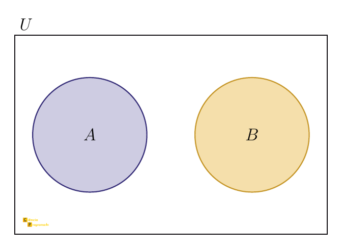
The simplest counting case occurs when the sets are disjoint: with no overlap, we just add.
If \(A \cap B = \emptyset\), then:
$$n(A \cup B) = n(A) + n(B)$$Generalizing: if \(A_1, A_2, \ldots, A_k\) are pairwise disjoint, then:
$$n(A_1 \cup A_2 \cup \cdots \cup A_k) = n(A_1) + n(A_2) + \cdots + n(A_k)$$The disjointness condition is essential. When there is an intersection, we need a more careful formula.
Inclusion-Exclusion Principle #
When the sets are not disjoint, the plain sum \(n(A) + n(B)\) counts the elements of the intersection twice. The Inclusion-Exclusion Principle (PIE; see the Wikipedia entry) fixes this systematically: it adds the individual sizes, subtracts the pairwise overlaps, adds back the triple ones, alternating signs until each element is counted exactly once.
Two sets #
The Venn diagram below helps visualize why the intersection is counted twice:
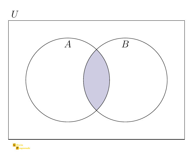
Why subtract the intersection? When adding \(n(A)\) and \(n(B)\), each element that belongs to both sets is counted twice, once when we count \(A\) and once when we count \(B\). Subtracting \(n(A \cap B)\) restores the correct count.
To derive the formula, we decompose the union into three disjoint regions:
$$A \cup B = (A - B) \cup (A \cap B) \cup (B - A)$$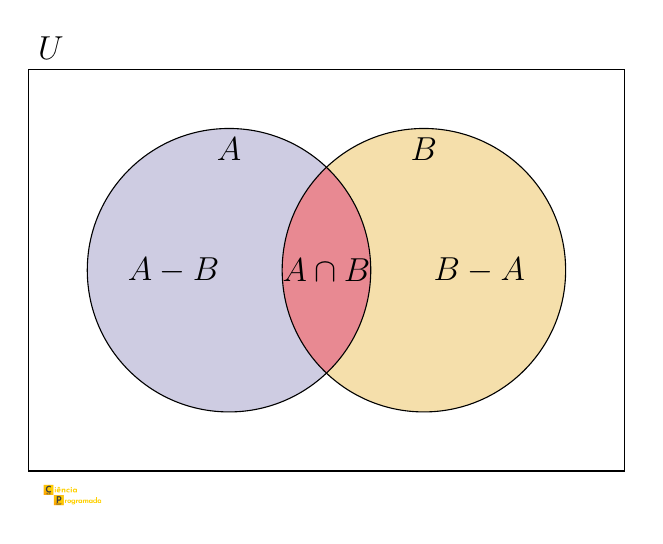
By the sum rule:
$$n(A \cup B) = n(A - B) + n(A \cap B) + n(B - A)$$But also:
$$n(A - B) = n(A) - n(A \cap B) \qquad \text{and} \qquad n(B - A) = n(B) - n(A \cap B)$$Substituting:
$$n(A \cup B) = \bigl[n(A) - n(A \cap B)\bigr] + n(A \cap B) + \bigl[n(B) - n(A \cap B)\bigr] = n(A) + n(B) - n(A \cap B)$$
Application in analytics: unique users (MAU)
Product teams track the MAU (Monthly Active Users): the number of unique users who accessed the platform in a given month. Suppose a streaming service records:
- \(n(Web) = 50{,}000\) visits through the browser
- \(n(App) = 40{,}000\) visits through the mobile app
Adding the two values directly would give 90,000, but many users access the service through both channels. If \(n(Web \cap App) = 15{,}000\), the real number of unique users is:
$$n(Web \cup App) = 50{,}000 + 40{,}000 - 15{,}000 = \mathbf{75{,}000}$$The Inclusion-Exclusion Principle corrects the double counting that inflates the metric, the same role it plays in theory.
Application in data engineering: deduplication in ETL pipelines (Extract, Transform, Load)
When integrating data from multiple sources, such as a CRM (Customer Relationship Management), an e-commerce platform, and a support system, a company needs to know how many unique customers it has in total. Each source keeps its own list and the same customers may appear in more than one system.
If \(n(\text{CRM}) = 12{,}000\), \(n(\text{Store}) = 8{,}000\), and \(n(\text{CRM} \cap \text{Store}) = 3{,}000\), the real number of distinct customers is:
$$n(\text{CRM} \cup \text{Store}) = 12{,}000 + 8{,}000 - 3{,}000 = \mathbf{17{,}000}$$In ETL pipelines, the PIE makes it possible to get the total of unique records directly from partial counts, without having to build or scan the full unified list.
Three sets #
The logic is the same: we add the individual sizes, subtract the pairwise overlaps (which were counted twice), and add back the triple overlap (which was subtracted once more than it should have been). The following figure identifies each of these regions in the Venn diagram:
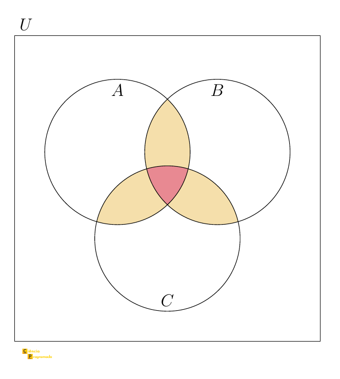
A direct derivation: apply the two-set case to \((A \cup B) \cup C\), using \(n(A \cup B)\) already worked out and the identity \((A \cup B) \cap C = (A \cap C) \cup (B \cap C)\).
To see why the formula is right, it is worth looking at the eight regions into which three sets divide the universe, numbered as in the article on Venn diagrams:
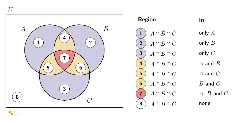
An element of region 7, which is in all three sets, is added 3 times in \(n(A) + n(B) + n(C)\), subtracted 3 times in the pairwise intersections, and added back 1 time in the triple one: \(3 - 3 + 1 = 1\). An element of regions 4, 5, or 6, which is in two sets, is added 2 times, subtracted 1 time, and does not appear in the triple one: \(2 - 1 = 1\). An element of regions 1, 2, or 3 is added once and appears in no other term, and those of region 8 enter no term at all. Each element of the union is counted exactly once.
Application in QA (Quality Assurance): unique bugs detected by three test suites
A quality team maintains three independent suites: unit tests (\(U\)), integration tests (\(I\)), and end-to-end tests (\(E\)). They want to know how many distinct bugs were found in total, without counting twice the bugs detected by more than one suite.
After a round of tests:
- \(n(U) = 45\), \(n(I) = 38\), \(n(E) = 27\)
- \(n(U \cap I) = 12\), \(n(U \cap E) = 8\), \(n(I \cap E) = 10\)
- \(n(U \cap I \cap E) = 3\)
Adding the individual totals would give 110, which is 27 more than the real number, exactly the number of bugs counted in duplicate (or triplicate) without the PIE correction.
Four sets #
The formula for four sets follows the same pattern, alternating signs:
$$ \begin{aligned} n(A_1 \cup A_2 \cup A_3 \cup A_4) ={}& n(A_1)+n(A_2)+n(A_3)+n(A_4) \\ &- n(A_1 \cap A_2)-n(A_1 \cap A_3)-n(A_1 \cap A_4) \\ &- n(A_2 \cap A_3)-n(A_2 \cap A_4)-n(A_3 \cap A_4) \\ &+ n(A_1 \cap A_2 \cap A_3)+n(A_1 \cap A_2 \cap A_4) \\ &+ n(A_1 \cap A_3 \cap A_4)+n(A_2 \cap A_3 \cap A_4) \\ &- n(A_1 \cap A_2 \cap A_3 \cap A_4) \end{aligned} $$General formula #
For \(k\) sets, the general formula of the Inclusion-Exclusion Principle is:
$$n\left(\bigcup_{i=1}^{k} A_i\right) = \sum_{i} n(A_i) - \sum_{i < j} n(A_i \cap A_j) + \sum_{i < j < l} n(A_i \cap A_j \cap A_l) - \cdots + (-1)^{k+1} n(A_1 \cap \cdots \cap A_k)$$The pattern is clear: we add the individual sizes, subtract the pairwise intersections, add the triple ones, and so on, alternating signs.
Classic example: derangements
In a gift exchange, \(n\) people put their gifts in a box and each one draws one. In how many draws does nobody get their own gift? A permutation like this, with no element in its original position, is called a derangement, and the number of them is denoted \(D_n\).
The total number of draws is \(n!\), the number of permutations of the \(n\) gifts. Let \(A_i\) be the set of draws in which person \(i\) gets their own gift; we want the draws outside \(A_1 \cup \cdots \cup A_n\).
- \(n(A_i) = (n-1)!\): the gift of \(i\) is fixed and the other \(n-1\) are permuted.
- The intersection of \(k\) of these sets fixes \(k\) gifts and has \((n-k)!\) elements. There are \(\binom{n}{k}\) ways to choose the \(k\) people, so the terms with \(k\) sets add up to \(\binom{n}{k}(n-k)! = \frac{n!}{k!}\).
By the PIE, with the sign \((-1)^{k+1}\) at each level, and taking the union out of the total:
$$D_n = n! - \sum_{k=1}^{n} (-1)^{k+1} \frac{n!}{k!} = n! \sum_{k=0}^{n} \frac{(-1)^k}{k!}$$For \(n = 4\): \(D_4 = 24 - 24 + 12 - 4 + 1 = 9\). You can check by listing the 24 permutations of \(1234\): only nine leave no digit in its place.
The sum \(\sum_{k} (-1)^k/k!\) converges to \(1/e\). The fraction of draws in which nobody gets their own gift tends to \(1/e\), about 36.8%. Rounded to one decimal place, it already gives 36.8% from 6 people on: it makes no difference whether the group has 10 or 10 thousand. More at Derangement.
Application in data science: Jaccard similarity
A widely used metric for comparing sets (in recommender systems, plagiarism detection, and document clustering) is the Jaccard similarity:
$$J(A, B) = \frac{n(A \cap B)}{n(A \cup B)}$$The denominator is rarely computed by materializing the union set. The Inclusion-Exclusion Principle lets us get it directly from counts:
$$n(A \cup B) = n(A) + n(B) - n(A \cap B)$$Thus, the similarity can be computed from three integers, without building the set \(A \cup B\) explicitly.
Example: two users of a streaming platform. User X watched the movies \(\{\text{A, B, C, D}\}\) and user Y watched \(\{\text{C, D, E, F}\}\). The movies in common are \(\{\text{C, D}\}\), so \(n(X \cap Y) = 2\). By the PIE:
$$n(X \cup Y) = 4 + 4 - 2 = 6 \implies J(X, Y) = \frac{2}{6} \approx 0.33$$The closer to 1, the more similar the tastes, without having to list all the movies watched by at least one of the two.
At large scale, techniques such as MinHash estimate \(J(A, B)\) directly, bypassing the PIE, taking advantage of the fact that the probability that two sets share the same minimum hash equals the Jaccard similarity itself.
Application in databases: cardinality estimation in query planners
SQL query optimizers (here, PostgreSQL’s) need to estimate, before executing,
how many rows each operation will return: this estimate determines the order
of the JOINs and which index to use. When a WHERE clause combines two
predicates with OR, the optimizer needs to estimate \(n(A \cup B)\), where
\(A\) and \(B\) are the sets of rows that satisfy each predicate
individually.
Without the Inclusion-Exclusion Principle, the optimizer would overestimate the result by adding the selectivities. With it, it uses:
$$n(A \cup B) \approx n(A) + n(B) - n(A \cap B)$$The estimates of \(n(A)\) and \(n(B)\) come from the column histograms and
the most-common-values lists kept by the database. For \(n(A \cap B)\), the
default behavior is to assume independence between the predicates: if 30% of
the rows satisfy predicate \(A\) and 20% satisfy \(B\), the optimizer
assumes the two criteria are unrelated and estimates that 6% of the rows
satisfy both, as if they were independent events (studied in probability).
Extended statistics (such as CREATE STATISTICS in PostgreSQL) refine this
estimate when the attributes are correlated, but require explicit
configuration.
The PIE therefore appears in the estimation of any query with OR
predicates in PostgreSQL, which computes \(s_1 + s_2 - s_1 s_2\) for the
selectivities \(s_1\) and \(s_2\), invisible to the developer but present in
the optimizer’s arithmetic.
Summary Table #
The formulas developed throughout the article, gathered for quick reference:
| Situation | Formula |
|---|---|
| Disjoint (\(A \cap B = \emptyset\)) | \(n(A \cup B) = n(A) + n(B)\) |
| Two sets | \(n(A \cup B) = n(A) + n(B) - n(A \cap B)\) |
| Three sets | \(n(A \cup B \cup C) = \sum n - \sum n(\cap_2) + n(\cap_3)\) |
| Complement | \(n(U - A) = n(U) - n(A)\) |
| Difference | \(n(A - B) = n(A) - n(A \cap B)\) |
In the three-set row, \(\sum n\) abbreviates the sum of the three individual sizes, \(\sum n(\cap_2)\) is the sum of the three pairwise intersections (\(n(A \cap B) + n(A \cap C) + n(B \cap C)\)), and \(n(\cap_3)\) is the triple intersection \(n(A \cap B \cap C)\). The complement and difference rows follow directly from the sum rule: just decompose the larger set into two disjoint parts and isolate the desired term.
Exercises #
Exercise 1: Divisibility in \(\{1, \ldots, 100\}\)
How many numbers from 1 to 100 are divisible by neither 2 nor 5?
Solution
Let \(C = \{1, \ldots, 100\}\), \(A\) = divisible by 2, \(B\) = divisible by 5.
- \(n(A) = 50\) (every second number)
- \(n(B) = 20\) (every fifth number)
- \(n(A \cap B) = 10\) (divisible by 10)
The ones divisible by neither 2 nor 5:
$$n(C) - n(A \cup B) = 100 - 60 = \mathbf{40}$$
Exercise 2: Proof
Let \(A\) and \(B\) be two subsets of \(U\) with \(B \subseteq A\). Prove, using the sum rule, that \(n(A - B) = n(A) - n(B)\).
Proof
Since \(B \subseteq A\), we have \(A \cup B = A\). We can rewrite \(A\) as the disjoint union \(A = (A - B) \cup B\). By the sum rule:
$$n(A) = n(A - B) + n(B)$$Therefore \(n(A - B) = n(A) - n(B)\). \(\blacksquare\)
Exercise 3: Multiples of 3 or 7 up to 100
How many integers from 1 to 100 are divisible by 3 or by 7?
Solution
Let \(A\) = multiples of 3, \(B\) = multiples of 7, in \(\{1,\ldots,100\}\).
- \(n(A) = \lfloor 100/3 \rfloor = 33\)
- \(n(B) = \lfloor 100/7 \rfloor = 14\)
- \(n(A \cap B)\) = multiples of \(\text{lcm}(3,7) = 21\): \(\{21, 42, 63, 84\}\), so \(n(A \cap B) = 4\)
Exercise 4: Multiples in \((1, 60)\)
Consider the integers from 2 to 59. Determine how many are:
(i) divisible by 2 and by 3 (ii) divisible by 2 or by 3 (iii) divisible by neither 2 nor 3
(iv) odd and divisible by 3, or divisible by 2 (v) divisible by 2, 3, or 5
Solutions
Let \(A\) = even numbers, \(B\) = multiples of 3, all in \((1,60)\) (excluding the endpoints):
\(n(A) = 29\), \(n(B) = 19\), \(n(A \cap B) = 9\) (multiples of 6).
(i) \(n(A \cap B) = \mathbf{9}\)
(ii) \(n(A \cup B) = 29 + 19 - 9 = \mathbf{39}\)
(iii) Total = 58 numbers. Not in \(A \cup B\): \(58 - 39 = \mathbf{19}\)
(iv) \(D\) = odd multiples of 3 = \(\{3,9,15,21,27,33,39,45,51,57\}\), \(n(D) = 10\). Since \(A \cap D = \emptyset\): \(n(A \cup D) = 29 + 10 = \mathbf{39}\)
(v) \(E\) = multiples of 5 in \((1,60)\) = \(\{5,10,\ldots,55\}\), \(n(E) = 11\). \(n(A \cap E) = 5\), \(n(B \cap E) = 3\), \(n(A \cap B \cap E) = 1\).
$$n(A \cup B \cup E) = 29+19+11-9-5-3+1 = \mathbf{43}$$
Exercise 5: Market research
200 people were asked about television prices: 40% asked about brand A, 35% about brand B, 10% about both, and 35% asked about neither brand. Determine:
(i) how many asked about A or B
(ii) how many asked about A and not about B
Solutions
In absolute values: \(n(A) = 80\), \(n(B) = 70\), \(n(A \cap B) = 20\).
(i) \(n(A \cup B) = 80 + 70 - 20 = \mathbf{130}\) people
(ii) \(n(A - B) = n(A) - n(A \cap B) = 80 - 20 = \mathbf{60}\) people
Sieve of Eratosthenes #
Exercises 1 and 3 and item (v) of 4 follow the same scheme: define a set by divisibility, compute its cardinality with \(\lfloor n/k \rfloor\), use the PIE to gather multiples of different primes without double counting and, when necessary, take the complement to count the elements that satisfy none of the conditions. This pattern, counting by the complement after applying the PIE, is recurrent in combinatorics.
These divisibility exercises apply exactly the same reasoning as the Sieve of Eratosthenes, the oldest known algorithm for finding all prime numbers up to a limit \(n\), proposed by the Greek mathematician Eratosthenes of Cyrene in the 3rd century BC.
A prime number is a natural number that has exactly two distinct natural divisors: the number 1 and itself.
The first primes are 2, 3, 5, 7, 11, 13, 17, 19, 23, 29, …
How it works #
Given an integer \(n > 1\), Eratosthenes’ method:
-
1
Build the list
Create a list of consecutive integers from 2 to \(n\). -
2
Start with 2
Let \(p = 2\), the smallest prime. -
3
Mark the multiples of \(p\)
Mark as composite all multiples of \(p\) starting from \(2p\): \(2p,\ 3p,\ 4p,\ \ldots\). \(p\) itself is not marked. -
4
Move on to the next prime
Find the smallest unmarked number in the list greater than \(p\). If there is none, stop. Otherwise, \(p\) takes this new value and go back to step 3. -
5
Read off the primes
When finished, the unmarked numbers are all the primes up to \(n\).
The central idea: every value taken by \(p\) is necessarily prime, because if it were composite, it would already have been marked as a multiple of some smaller prime. Note that, in this basic algorithm, some numbers may be marked more than once: 15, for example, is marked both when processing \(p = 3\) and when processing \(p = 5\).
Optimization: in step 3, it is enough to start at \(p^2\) instead of \(2p\), since every multiple \(k \cdot p\) with \(k < p\) has a prime factor \(q \leq k < p\) by which it was already marked in an earlier stage. With that, it is also enough to run step 3 while \(p^2 \leq n\): upon reaching a \(p\) with \(p^2 > n\), all the numbers still unmarked are necessarily prime.
For example, when processing \(p = 5\), the multiples before \(p^2 = 25\) have already been marked: \(10 = 2 \cdot 5\) was marked when \(p = 2\); \(15 = 3 \cdot 5\), when \(p = 3\); \(20 = 4 \cdot 5 = 2^2 \cdot 5\), again when \(p = 2\). The first multiple of 5 that can still be unmarked is \(25 = 5^2\), hence the start at \(p^2\).
The animation below illustrates the complete algorithm with the optimization applied, for all primes below 121:

Example for \(n = 30\), with primes in bold and composites struck through:
| 2 | 3 | 5 | 7 | 11 | |||||
| 13 | 17 | 19 | |||||||
| 23 | 29 |
With \(p = 2\): 4, 6, 8, …, 30 are marked. With \(p = 3\): 9, 15, 21, 27 are marked (the even numbers were already marked). With \(p = 5\): 25 is marked. The next prime would be \(p = 7\), but \(7^2 = 49 > 30\): the only multiples of 7 in the range (14, 21, and 28) are already marked by smaller primes (2 and 3). All the numbers still unmarked are prime. Ten remain: the primes from 2 to 29.
Algorithm #
The pseudocode below directly incorporates the \(p^2\) optimization:
Input:  integer n > 1
Output: all primes from 2 to n

A ← array[2..n] initialized with True

For i from 2 to √n:
    If A[i] is True:
        For j from i² to n with step i:
            A[j] ← False

Return all i with A[i] = True
The flowchart below represents the same algorithm visually:
flowchart TD
    A([Start]) --> B["A ← array[2..n] = True
i ← 2"]
    B --> C{"i ≤ √n ?"}
    C -->|No| G[/"Return all i
with A[i] = True"/]
    G --> H([End])
    C -->|Yes| D{"A[i] = True ?"}
    D -->|No| F["i ← i + 1"]
    F --> C
    D -->|Yes| E["j ← i²"]
    E --> I{"j ≤ n ?"}
    I -->|No| F
    I -->|Yes| J["A[j] ← False"]
    J --> K["j ← j + i"]
    K --> I
In the pseudocode, the same optimization appears from two angles: the inner loop starts at \(i^2\) because earlier multiples have already been marked; the outer loop stops at \(\sqrt{n}\) because, when \(i > \sqrt{n}\), we have \(i^2 > n\), and there is no multiple of \(i\) from \(i^2\) on within the range. The two conditions are equivalent.
Time complexity: \(O(n \log \log n)\). The intuition: for each prime \(p \leq n\), the inner loop performs about \(n/p\) steps. The total cost is proportional to \(n \sum_{p \leq n} 1/p\), and by Mertens' theorem this sum grows like \(\log \log n\), much more slowly than \(\log n\) (the full harmonic series). In practice, for \(n = 10^9\), \(\ln \ln n \approx 3\): the algorithm is almost linear.
Space complexity: the pseudocode above allocates an array of \(n\) positions, hence \(O(n)\), infeasible for \(n = 10^9\). The Segmented Sieve is a variant that reduces the space to \(O(\sqrt{n})\) without increasing the time complexity. The idea in two phases: first, run the classic sieve up to \(\sqrt{n}\) to obtain all the small primes (this array fits in \(O(\sqrt{n})\)); then, divide \([2, n]\) into blocks of size \(\approx \sqrt{n}\) (sized to fit in the processor’s cache memory) and process one block at a time, marking the multiples of the small primes that fall in that range. The resulting pseudocode is longer than the one above, but the principle is the same.
Additions only: the sieve advances by counting in increments of \(p\), with no divisions or divisibility tests. This is what distinguishes it from trial division, which tests each candidate individually, and is the basis of its efficiency.
The connection with the PIE #
Why does the sieve work mathematically? Every composite number \(m \leq n\) has at least one prime factor \(p \leq \sqrt{m} \leq \sqrt{n}\), so every composite falls in some \(A_p\) and is eliminated. What remains are the primes.
Back to the example with \(n = 30\): \(21 = 3 \times 7\) is composite and \(\sqrt{21} \approx 4.6\), so it has a prime factor \(\leq 4.6\) (indeed, 3) and was eliminated when \(p = 3\). Meanwhile \(25 = 5^2\) has \(\sqrt{25} = 5\), with prime factor \(5 \leq 5\), eliminated when \(p = 5\). No composite escapes: there is always a prime factor small enough to have marked it before the outer loop ends.
Eliminating the multiples of a prime \(p\) amounts to defining:
$$A_p = \{k \in \{1, \ldots, n\} : k \text{ is a multiple of } p\}$$In words: \(A_p\) is the set of all integers from 1 to \(n\) that the sieve would mark when processing the prime \(p\). For example, for \(p = 3\) and \(n = 30\), we have \(A_3 = \{3, 6, 9, 12, \ldots, 30\}\). Each step of the algorithm does nothing more than build this set and strike out its elements.
The survivors of the sieve are the integers from 1 to \(n\) that belong to no \(A_p\), that is, the complement of the union of all these sets. Calling \(p_1, \ldots, p_r\) the primes up to \(\sqrt{n}\), the count of the survivors is:
$$n - n(A_{p_1} \cup \cdots \cup A_{p_r})$$(The number 1 also survives, since it is not divisible by any prime; \(p_1, \ldots, p_r\) themselves are excluded, since each \(p_i\) belongs to its own \(A_{p_i}\). The sieve starts at 2, which takes care of both in practice.)
To compute \(n(A_{p_1} \cup \cdots \cup A_{p_r})\), we apply the PIE. This requires knowing the cardinalities of the individual sets and of the intersections. The key is that the intersection of two sets of multiples is itself a set of multiples: \(A_p \cap A_q\) contains exactly the integers divisible by \(p\) and by \(q\), that is, the multiples of the product \(pq\) (which is the lcm of two distinct primes). Therefore:
- The cardinality of \(A_p\) is the number of multiples of \(p\) up to \(n\), given by the integer part \(\lfloor n/p \rfloor\).
- The cardinality of the intersection \(A_p \cap A_q\) is the number of multiples of \(pq\) up to \(n\), given by \(\lfloor n/(pq) \rfloor\).
You computed exactly this in item (v) of Exercise 4: with \(A\) = even numbers, \(B\) = multiples of 3, and \(E\) = multiples of 5 in the range \((1, 60)\), you applied the PIE to \(A_2 \cup A_3 \cup A_5\) and got 43. The exercise stopped there, but the sieve takes one more step: it takes the complement, \(58 - 43 = 15\), to count the survivors (the numbers from 2 to 59 not divisible by 2, 3, or 5, which include all primes greater than 5 in that range). The Sieve of Eratosthenes is this reasoning generalized to any \(n\) and any set of primes.
The Sieve of Eratosthenes is an algorithm: it iteratively marks multiples and counts what remains. What we did in this section was different: we expressed the same result as a closed-form formula via the PIE, directly computing \(n - n(A_{p_1} \cup \cdots \cup A_{p_r})\) without simulating the process step by step. This mathematical formalization is historically known as the Legendre sieve, named in honor of Adrien-Marie Legendre, who in the 19th century made explicit the PIE structure behind the sieve. The central formula of the method is called Legendre’s identity, and it generalizes the expression above using the Möbius function \(\mu(d)\). This function encodes exactly the alternating sign pattern of the PIE: for a number \(d\) that is a product of \(k\) distinct primes, \(\mu(d) = (-1)^k\); if \(d\) contains some squared factor, \(\mu(d) = 0\). With this, the whole PIE expansion (add the individual ones, subtract the pairs, add the triples, and so on) condenses into a single sum, which already gives the count of the survivors:
$$n - n(A_{p_1} \cup \cdots \cup A_{p_r}) = \sum_{d \mid P} \mu(d) \left\lfloor \frac{n}{d} \right\rfloor$$where \(P = p_1 \cdot p_2 \cdots p_r\) is the product of the primes up to \(\sqrt{n}\) and the sum runs over all divisors \(d\) of \(P\), including \(d = 1\). It is this term that plays the role of the initial \(n\): \(\mu(1) \lfloor n/1 \rfloor = n\). The prime divisors (\(\mu = -1\)) subtract the individual sets, the products of two primes (\(\mu = +1\)) add back the pairwise intersections, and so on. It is the same arithmetic as the PIE, rewritten compactly.
For \(n = 30\), the primes up to \(\sqrt{30}\) are 2, 3, and 5, and \(P = 30\). The eight divisors of 30 give:
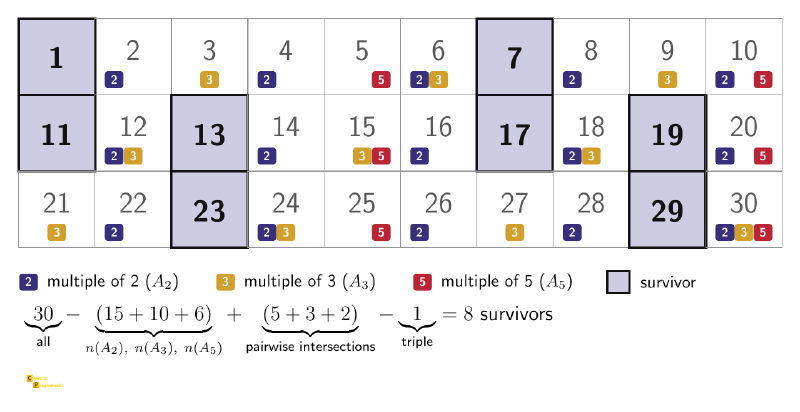
$$\underbrace{30}_{d=1} - \underbrace{15 - 10 - 6}_{d \in \{2, 3, 5\}} + \underbrace{5 + 3 + 2}_{d \in \{6, 10, 15\}} - \underbrace{1}_{d=30} = 8$$These are exactly the eight survivors \(\{1, 7, 11, 13, 17, 19, 23, 29\}\): 1 is in, and the primes 2, 3, and 5 are out, as explained above.
The figure below puts this computation on the numbers themselves. Each integer from 1 to 30 gets a mark for each set \(A_2\), \(A_3\), \(A_5\) it belongs to, and those left with no mark are the survivors. Counting the marks of each color gives \(15\), \(10\), and \(6\). The pairwise intersections add up to \(5 + 3 + 2 = 10\): they are the seven cells with two marks (6, 10, 12, 15, 18, 20, and 24) plus 30, which has three marks and is therefore in all three pairwise intersections, and is, on its own, the triple one.
Next steps #
With cardinality and the Inclusion-Exclusion Principle, we close the theoretical block of this stage of the series: defining, representing, operating on, and counting sets without double counting.
In the next article of the series, the same language appears in code: we will
see how membership, inclusion, union, intersection, and cardinality translate
directly into Python using set and frozenset, connecting theory to
practice.
See you there!


