

In the previous article, Memory Hierarchy, we saw that DRAM is too slow for the processor and that SRAM, although fast, is too expensive for large volumes. We ended with the principles of temporal and spatial locality: the empirical observation that real programs tend to reuse the same data and to access neighboring addresses. These are exactly the principles that make the cache memory viable, and that is what we are going to explore now.
In this article you will understand:
- the speed bottleneck between CPU and DRAM and why it grows over time;
- how the principles of locality translate into hit and miss;
- the three types of mapping that define where a block of MM can go in the cache;
- the algorithms that decide which block to replace when the cache is full;
- the write policies and how they keep cache and MM consistent;
- the physical organization of memory in chips: 1D versus 2D.
The CPU/MM Speed Problem #
DRAM transfers data to the CPU at a speed lower than the one at which the processor can consume it. When this happens, the CPU has to wait, inserting wait states (waiting cycles) and sitting idle for part of the time.
Historically, processor performance has evolved faster than the latency and bandwidth of main memory. This mismatch was one of the main reasons for the appearance of cache memory.
It even has a name: the memory wall, a phrase made famous by the paper Hitting the Memory Wall: Implications of the Obvious, by Wulf and McKee, in 1995. And there are numbers behind it. From the mid-1980s on, processor performance started to grow at around 50% per year, while DRAM latency improved by something like 7% per year. Two different exponential rates do not drift apart slowly. That is why, in a current processor running at a few gigahertz, a main memory access costs on the order of two hundred cycles: two hundred opportunities to do work that the CPU spends waiting. Memory got better, but the processor got better much faster, and the gap has never stopped growing.
The figure below shows this divergence since 1980. The vertical axis is logarithmic: each grid line is worth ten times the previous one, and that is the only reason the two curves fit on the same chart. On a common scale, the memory curve would be a line practically glued to zero.
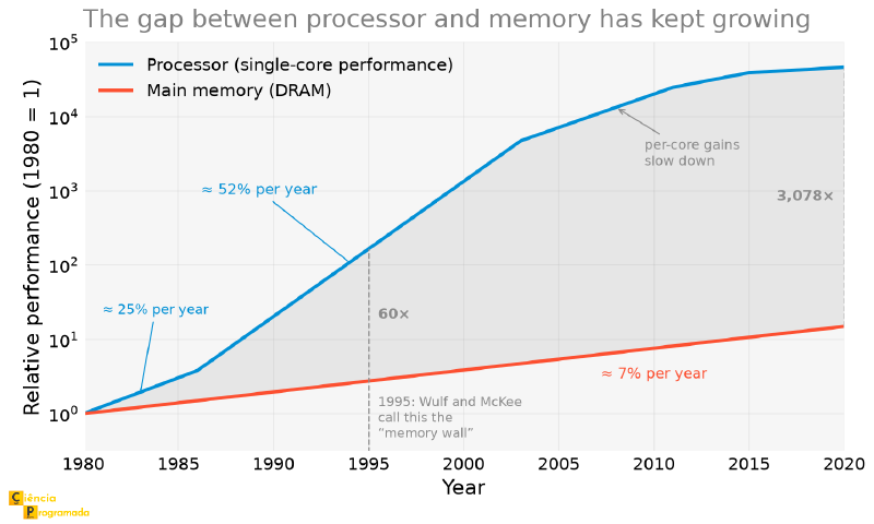
Two things can be read from the figure besides the gap itself. The first is that it was already tens of times when the term was coined, in 1995. The second is the processor curve flattening from the mid-2000s: the performance gain per core slowed down, for reasons that the last article of the series explains and that pushed the industry toward multicore processors.
Who invented the cache
The idea appears in 1965, in a two-page paper by Maurice Wilkes called Slave Memories and Dynamic Storage Allocation. Wilkes proposed a small, fast memory, which he called a slave memory, keeping copies of what main memory held, managed entirely by the hardware, without the program knowing it existed. That is the definition of a cache, three years before the name caught on.
The first commercial machine to ship with one was the IBM System/360 Model 85, in 1968, with 16 KB of high-speed buffer, the term IBM used. It was around then that “cache” became the standard word, borrowed from the French cacher, to hide: a memory whose purpose is to be invisible to the programmer.
In theory, a simple solution would be to build the entire main memory with SRAM, which is much faster. In practice, this is unfeasible: SRAM takes up more area on the chip and costs much more per stored bit. The engineering solution was to place a small, very fast memory between the CPU and the DRAM: the CPU cache.
Why does the cache work?
The cache is only efficient because real programs exhibit locality of reference. Without this empirically observed behavior, the cache would bring no performance gain.
Principles of Locality #
The efficiency of the cache depends on an observable behavior of real programs called locality of reference. Two complementary principles describe this behavior:
| Principle | Definition | Practical example |
|---|---|---|
| Temporal | If the program accesses word \(X\), there is a high probability of accessing \(X\) again soon | Control variable in a for loop |
| Spatial | If the program accesses word \(X\), there is a high probability of accessing nearby words next | Sequential instructions; consecutive elements of an array |
The cache exploits both: on a miss, it loads a whole block of contiguous cells (spatial locality) and keeps that block in its slots for as long as possible (temporal locality). For most programs, this means that the vast majority of subsequent accesses result in a hit, with no need to search the DRAM. But how exactly does the CPU decide whether the data is in the cache or whether it has to “go down” to main memory?
How the Cache Works #
The rule of computer architecture is: the CPU always tries to fetch instructions and data from the cache first. On each access, the hardware checks whether the desired block is already present in it:
graph TD
    A["CPU requests instruction or data"]
    B{"Block present
in the cache?"}
    H["HIT
Data transferred cache→CPU
at high speed"]
    M["MISS
Whole block transferred MM→cache
then word→CPU"]
    F["Data delivered to the CPU"]

    A --> B
    B -->|"Yes"| H --> F
    B -->|"No"| M --> F
| Situation | What happens | Transfer granularity |
|---|---|---|
| Hit | Data found in the cache | Word cache → CPU |
| Miss | Data not found | Block MM → cache; then word → CPU |
Block transfer on a miss exploits spatial locality: if a word was needed now, there is a good chance that neighboring words will be accessed next too.
What a Hit Rate Is Worth #
The fraction of accesses that result in a hit is called the hit rate, and is usually represented by \(h\). It is the number that decides whether the cache was worth it, because the average access time seen by the processor is a weighted average of the two possible paths:
$$T_m = h \cdot T_c + (1 - h) \cdot T_{MM}$$where \(T_c\) is the cache access time and \(T_{MM}\) the main memory access time. It is worth putting numbers on this, using the orders of magnitude from the previous article, \(T_c = 1\) ns and \(T_{MM} = 80\) ns:
$$T_m = 0.95 \times 1 + 0.05 \times 80 = 0.95 + 4 = 4.95\ \text{ns}$$With a 95% hit rate, the processor sees a 4.95 ns memory, about 16 times faster than plain DRAM, using a cache that holds a tiny fraction of the total. This result is what justifies the existence of the cache.
The same calculation shows why cache design is so sensitive: at a 90% hit rate the average time rises to 8.9 ns, almost double. Every percentage point of hit rate lost is costly, because the term it feeds is the slower of the two.
80 ns
Plain DRAM
4.95 ns
95% hit rate
8.9 ns
90% hit rate
Cache Types and Levels #
A useful distinction is this:
- when we talk about cache memory in this article, the main focus is the processor cache, built to reduce the cost of accessing main memory;
- when we talk about speeding up disk access, in current systems the topic is commonly found under names such as file system cache or page cache in RAM, and not necessarily as “disk cache” in the classic sense.
But the general idea is always the same: use a faster layer to cushion the cost of accessing a slower layer.
| Type | Accelerated relationship | Typical implementation |
|---|---|---|
| CPU cache | CPU ↔ Main Memory | SRAM |
| File system cache | RAM ↔ secondary storage | DRAM |
| Level | Typical location | Speed | Typical capacity |
|---|---|---|---|
| L1 | Inside the processor core | Maximum | Tens of KB |
| L2 | Inside the processor | Very high | Hundreds of KB to a few MB |
| L3 | Inside the processor, usually shared | High | Several MB |
Split cache: in many architectures, instructions and data are kept in separate caches, which reduces conflicts and improves internal parallelism.
Historical evolution of the cache levels
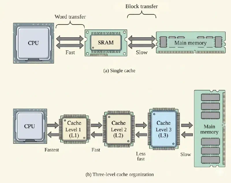
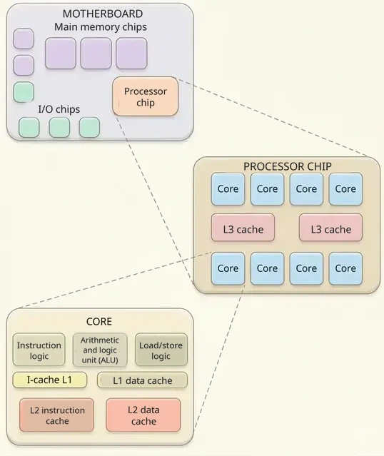
In older architectures, it was common for only the L1 cache to sit inside the processor, while the L2 could be outside it, for example on the motherboard or in a separate chip. In current processors, it is most common for L1, L2, and L3 to be integrated into the processor itself. In many cases, L1 and L2 are private to each core, while the L3 is shared. The figures below illustrate this evolution:
The Four Cache Design Elements #
Designing a cache memory requires hardware engineers to balance cost, complexity, and performance. This balance involves four elements:
| # | Element | Issue involved |
|---|---|---|
| 1 | Size | What is the total capacity? (affects cost, hit rate, and access time) |
| 2 | Mapping function | How is a block of MM associated with a cache line? |
| 3 | Replacement algorithm | Which block to remove when a miss occurs and there is no free line? |
| 4 | Write policy | How to keep cache and MM consistent on write operations? |
Essential terminology:
- Block: unit of transfer between MM and cache; contains \(K\) contiguous cells
- Line: space in the cache that holds a block
- \(B\) = total number of blocks in MM
- \(Q\) = number of lines in the cache, where \(Q \ll B\)
Mapping Functions #
Direct Mapping #
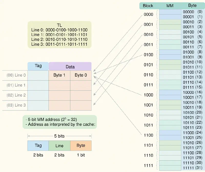
Each block of MM has a single possible cache line, determined by:
$$\text{cache line} = \text{block number} \bmod Q$$The figure below illustrates direct mapping, where MM blocks are mapped to specific cache lines. Note that different blocks can compete for the same line, which can lead to frequent conflicts.
Division of the \(E\)-bit address:
| Field | No. of bits | Function |
|---|---|---|
| Tag | \(E - \log_2 Q - \log_2 K\) | Identifies which of the \(B/Q\) blocks is in that line |
| Line no. | \(\log_2 Q\) | Selects the cache line |
| Word in block | \(\log_2 K\) | Selects the cell/word within the block |
Numerical example: direct mapping
- MM = 4 Gbytes addressable → \(E = 32\) bits
- Cache: \(Q = 1024\) lines, \(K = 64\) bytes/block
- Line bits: \(\log_2 1024 = 10\)
- Word bits: \(\log_2 64 = 6\)
- Tag bits: \(32 - 10 - 6 = 16\)
- Total blocks: \(B = 4G / 64 = 64M\) → \(\mathbf{65{,}536}\) blocks mapped to each line!
| Aspect | Direct mapping |
|---|---|
| Advantage | Simple and cheap to implement |
| Disadvantage | Block conflict: two blocks in the same line replace each other, even if other lines are free |
To solve this constant “crushing” problem of direct mapping, engineers proposed the opposite extreme: giving the block total freedom.
Associative Mapping (fully associative) #
A block can be placed in any cache line.
The figure below shows associative mapping, where MM blocks can be stored in any cache line, completely eliminating block conflicts. However, this requires more complex search logic to locate a specific block.
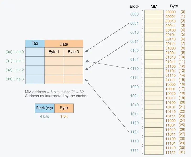
Division of the address:
| Field | No. of bits | Function |
|---|---|---|
| Tag | \(E - \log_2 K\) | Identifies the block (= block number in MM) |
| Word in block | \(\log_2 K\) | Selects the word within the block |
To locate a block, the controller compares the tag with all \(Q\) lines simultaneously (parallel hardware).
| Aspect | Associative mapping |
|---|---|
| Advantage | Completely eliminates block conflicts |
| Disadvantage | Complex and expensive search logic; impractical for large caches |
Since the parallel search across all lines produces very expensive hardware, the industry had to find a middle ground between the rigidity of direct mapping and the high cost of associative mapping.
Set-Associative Mapping (set-associative) #
A compromise between the two previous ones. The cache is divided into \(C\) sets of \(D\) lines each:
$$Q = C \times D \qquad\qquad \text{set} = \text{block number} \bmod C$$The figure below illustrates set-associative mapping, where the cache is divided into sets, and each MM block is mapped to a specific set, but can occupy any line within that set. This reduces block conflicts compared to direct mapping, while keeping the search complexity more manageable than in fully associative mapping.
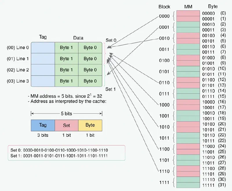
Division of the address:
| Field | No. of bits | Function |
|---|---|---|
| Tag | \(E - \log_2 C - \log_2 K\) | Identifies the block within the set |
| Set no. | \(\log_2 C\) | Selects the set |
| Word in block | \(\log_2 K\) | Selects the word |
The tag is compared only with the \(D\) lines of the set, not with the whole cache.
graph LR
    B0["MM: Block 0
(0 mod C = 0)"]
    BC["MM: Block C
(C mod C = 0)"]
    B1["MM: Block 1
(1 mod C = 1)"]
    BC1["MM: Block C+1
(C+1 mod C = 1)"]

    subgraph S0["Set 0: D lines"]
        L00["Line 0"]
        L01["Line 1"]
    end

    subgraph S1["Set 1: D lines"]
        L10["Line 0"]
        L11["Line 1"]
    end

    B0 --> L00
    BC --> L01
    B1 --> L10
    BC1 --> L11
Comparison of the Three Techniques #
| Technique | Flexibility | Complexity | Cost | Block conflict |
|---|---|---|---|---|
| Direct | Low (1 fixed line per block) | Low | Low | Frequent |
| Associative | Total (any line) | High | High | None |
| Set-assoc. | Medium (\(D\) lines per set) | Medium | Medium | Reduced |
Most widely used technique in modern processors
Set-associative mapping with \(D = 2\), \(4\), or \(8\) ways dominates current designs. It balances the low cost of direct mapping with the flexibility of fully associative mapping.
The Three Types of Miss #
With the three mappings on the table, we can classify the misses, and the classification matters, because each type is fought in a different way. The taxonomy is known as the three C’s, made canonical by Mark Hill and Alan Jay Smith in the late 1980s:
| Type | Why it happens | How to attack it |
|---|---|---|
| Compulsory (or cold start) | It is the first access to that block; it was never in the cache | Unavoidable by definition: it can only be anticipated, with prefetch |
| Capacity | The set of data the program uses is larger than the entire cache | Larger cache, or rewrite the program to work in smaller pieces |
| Conflict | The block fit in the cache, but the mapping forced the eviction of another one that was still useful | More associativity |
The third is the block conflict that appears throughout the direct mapping section, now with a name of its own. And the classification explains the comparison table at once: in fully associative mapping the conflict miss does not exist, because no block is forced to go to a specific place. What remains are the compulsory ones, which nobody avoids, and the capacity ones, which only a larger cache solves.
Let us see how to compute the address fields for each technique in a concrete example:
Example: address fields in the three types of mapping
A machine can address 4 Gbytes of physical memory with 2-byte cells, organized in 1 Kbyte blocks. The cache holds 2K lines (one block per line). Compute the address fields for the three types of mapping.
Given: 4 Gbytes; cell = 2 bytes → \(N = 2\text{G} = 2^{31}\) cells → \(E = 31\) bits. Block = 1 Kbyte = 512 cells → \(B = 2^{31}/2^9 = > 2^{22} = 4\text{M}\) blocks. Cache: \(Q = 2\text{K} = 2^{11}\) lines.
Direct mapping:
$$\underbrace{11}_{\text{tag}} \underbrace{11}_{\text{line}} \underbrace{9}_{\text{word}} = 31\ \text{bits}$$- line field: \(Q = 2^{11}\) → \(\mathbf{11}\) bits; word field: \(2^9\) → \(\mathbf{9}\) bits
- tag field: \(B/Q = 2^{22}/2^{11} = 2^{11}\) → \(\mathbf{11}\) bits
Fully associative mapping:
$$\underbrace{22}_{\text{tag}} \underbrace{9}_{\text{word}}$$- tag field: \(B = 2^{22}\) → \(\mathbf{22}\) bits; word field: \(\mathbf{9}\) bits
Set-associative mapping (\(D = 4\)):
- \(C = Q/D = 2^{11}/4 = 2^9\) sets $$\underbrace{13}_{\text{tag}} \underbrace{9}_{\text{set}} \underbrace{9}_{\text{word}} = 31\ \text{bits}$$
- set field: \(\mathbf{9}\) bits; tag field: \(B/C = 2^{22}/2^9 = 2^{13}\) → \(\mathbf{13}\) bits; word field: \(\mathbf{9}\) bits
The interpretation of the fields becomes clearer when we look at what happens on a hit and a miss for a specific address:
Example: hit and miss for a given address
A machine with 32 Gbytes of physical memory has 4-byte cells and a cache
with 16 M blocks (1 block per line, 8 cells per block). For address 2
(binary: 0000...010), what characterizes a hit and a miss in each
type?
Given: \(N = 8\text{G} = 2^{33}\) → \(E = 33\) bits. Block = 8 cells → \(B = 2^{33}/2^3 = 2^{30}\) blocks. Cache: \(Q = 2^{24}\). Word field: \(2^3\) → \(\mathbf{3}\) bits.
It is worth noting that this cache has \(2^{24}\) lines of 32 bytes each, that is, 512 MB, two orders of magnitude above any real L3. The values were chosen so that the powers of 2 come out round; the procedure is identical at any scale.
Direct mapping: line field: \(\mathbf{24}\) bits; tag: \(2^{30}/2^{24} =
> 2^6\) → \(\mathbf{6}\) bits. Address 2: 000000 | 000...000 | 010.
- Hit: goes to the line given by the 24 middle bits, compares the tag; if equal, direct access.
- Miss: different tags → whole block transferred from MM.
Fully associative: tag field: \(\mathbf{30}\) bits.
- Hit: searches all lines in parallel; if any tag matches → hit.
- Miss: no line has the tag → block transferred.
Set-associative (\(D = 4\)): \(C = 2^{24}/4 = 2^{22}\); set field: \(\mathbf{22}\) bits; tag: \(2^{30}/2^{22} = 2^8\) → \(\mathbf{8}\) bits.
- Hit: finds the set by the 22 middle bits; compares the tag in the 4 lines.
- Miss: none of the 4 lines has the tag → block transferred.
Replacement Algorithms #
When a miss occurs and there is no free line available, the controller has to decide which old block will be removed to make room for the new one.
This decision only exists in cases where a choice is possible, that is, in associative mapping and set-associative mapping. In direct mapping, the new block always replaces the block that already occupies the single line compatible with it.
| Algorithm | Strategy | Note |
|---|---|---|
| LRU (Least Recently Used) | Removes the block unaccessed for the longest time | Tends to work well when there is strong temporal locality |
| FIFO | Removes the block loaded the longest ago | Simple to implement |
| LFU (Least Frequently Used) | Removes the block with the fewest accumulated accesses | May preserve old blocks that are no longer useful |
| Random | Random choice | Simple hardware |
About LRU
LRU is usually a good strategy because it approximates the principle of temporal locality. Still, real implementations often use approximations of LRU, especially in larger caches, to reduce the cost of the control hardware.
Write Policies #
Reading from the cache is simple: just check whether the block is present. Writing is more delicate, because an update made in the cache can leave Main Memory with an outdated copy. The write policies define how this synchronization will be handled.
Write Through #
- Every write updates the cache and Main Memory at the same time
- Keeps MM always coherent with the cache
- Simple to understand and implement
- Can greatly increase write traffic to MM
Write Back #
- The write updates only the cache
- The block receives a modification mark (dirty bit)
- MM is only updated when that block is removed from the cache
- Reduces write traffic, but requires additional control
Write Once, Which Is Not a Write Policy #
Textbooks usually present write once as a third policy, on the same level as the two previous ones. The behavior described is this:
- the first write to a block is done as write through;
- subsequent writes are treated as write back.
But the classification is misleading. Write once was proposed by James Goodman in 1983 as a cache coherence protocol, a different category. The problem it solves is not keeping main memory up to date; it is warning the other caches that that block has changed. The first write goes to MM precisely because it is the bus that the other cores observe: there it works as a signal, not as synchronization.
And it is one of the predecessors of the protocol that dominates current systems, MESI, a name formed from the four states that each cache line can assume: Modified, Exclusive, Shared, and Invalid. That is the term to search for when the subject is coherence, and it is the one that reappears in the last article of the series, when dealing with multiprocessors.
Cache coherence in multicore systems
In systems with multiple cores or multiple processors, each core can keep local copies of the same block in its own cache. If one of them modifies that block, the other copies may become outdated. This is the problem of cache coherence.
Write policies influence this scenario, but do not solve it alone: what solves it is a coherence protocol implemented in hardware, and in the vast majority of current processors that protocol is MESI or one of its variants.
The classic literature, as pointed out in William Stallings’ book, shows that approximately 15% of all memory operations are writes, since the vast majority of accesses consist of reads to fetch instructions and data. This number has been used as an argument that write through would suffice in most cases, but current practice is subtler, and depends on the level of the hierarchy.
Some microarchitectures use write through on the L1 toward the L2, like the data L1 of the AMD Bulldozer: the distance between the two is short, a write buffer absorbs the traffic, and the simplicity pays off. The L2 and L3, on the other hand, are typically write back, for a reason that the memory wall explains well. The scarcest resource in the system is DRAM bandwidth, and writing straight to that level would waste bandwidth on values that will still be overwritten in the cache itself before anyone needs them. Accumulating the writes and paying once, when the line is evicted, is what keeps the memory bus free for what matters.
Physical Organization of Memory #
The 1D and 2D physical organization is an important memory implementation detail, but here it should be understood as a hardware backdrop for memory chips in general, and not as the core of the logical operation of the cache.
Whether we are talking about Cache or Main Memory, at the lowest hardware level, billions of bits need to be stored in transistors inside silicon chips. The way these circuits are designed so that an address finds its physical cell happens in two main ways:
Type 1D: Linear Selection #
- The address directly drives one of \(2^E\) decoder outputs
- Conceptually simple
- Scales poorly for large values of \(E\)
Type 2D: Row/Column Matrix #
- The address is split between row and column
- The cell is selected at the intersection between them
- Drastically reduces the size of the decoders
Example with \(E = 14\) bits:
$$7\ \text{row bits} + 7\ \text{column bits} \implies 128 \times 128 = 16K\ \text{cells}$$
graph TD
    ADDR["Address: 14 bits"]
    DL["Row Decoder
7 bits → 128 outputs"]
    DC["Column Decoder
7 bits → 128 outputs"]
    CEL["Selected cell
Row × column intersection"]

    ADDR -->|"bits 13 to 7"| DL
    ADDR -->|"bits 6 to 0"| DC
    DL --> CEL
    DC --> CEL
| Organization | Decoder outputs (\(E = 14\)) | Hardware efficiency |
|---|---|---|
| 1D (linear) | \(2^{14} = 16{,}384\) outputs | Low |
| 2D (matrix) | \(2^7 + 2^7 = 256\) outputs | High |
Conclusion and Next Articles #
The cache is a small, fast, expensive component that, when well placed in the memory hierarchy, multiplies the efficiency of the whole system without requiring changes to the software. Each design decision (type of mapping, replacement algorithm, write policy) is a compromise between performance, cost, and implementation complexity.
For those who want to go deeper, much deeper, the canonical reference on the subject is What Every Programmer Should Know About Memory, by Ulrich Drepper (2007). It is about a hundred open pages that start more or less where this article ends: real measurements, and the effect of each cache decision on real code.
In the next article, we will talk about the CPU. The components that make up the central processing unit, how they are interconnected, and what happens step by step when an instruction is fetched and executed.
See you then.


