

In the previous article, Data Representation, we saw how the computer encodes characters, integers, and floating-point numbers as bit patterns. But a program is not just data: it is a sequence of instructions that tell the processor what to do with that data. How are these instructions encoded? Where does the processor find the operands they need?
These questions are answered by the ISA (Instruction Set Architecture) and by the addressing modes it defines. The ISA is the meeting point between hardware and software: everything a program does must be expressed in terms the processor understands.
The ISA: the contract between hardware and software #
The ISA (Instruction Set Architecture) is the interface between hardware and software. It defines the set of instructions the processor understands and the model visible to compilers, assemblers, operating systems, and programs.
The ISA specifies, among other things:
- the instruction format;
- the supported data types;
- the addressing modes;
- the registers and their roles;
- the set of operations the CPU executes natively.
It is useful to think of the ISA as a compatibility contract: programs translated for an ISA only run directly on processors that implement that ISA, except through emulation, binary translation, or virtual machines.
ISA is not the same thing as microarchitecture
Two processors can implement the same ISA and still be very different internally. This is the case with different x86-64 CPUs from Intel and AMD: the software sees the same ISA, but the internal hardware can vary a lot.
Programming languages and ISA
Not every high-level language turns directly into instructions of the machine’s ISA.
- In natively compiled languages, such as C and C++, the compiler usually generates machine code for the target ISA.
- In languages or platforms such as Java and Python, there may be intermediate steps, such as bytecode, a virtual machine, or JIT compilation, before the final execution on the hardware.
Even so, ultimately, the actual execution always ends in instructions of the ISA implemented by the processor.
ISAs in the market today
The x86-64 family remains dominant on desktops and many servers. The ARM family now goes far beyond smartphones, also appearing in embedded systems, laptops, the cloud, and data centers. RISC-V, in turn, has gained relevance for being an open ISA, especially in research, teaching, and embedded systems.
A useful classification of instructions #
A didactic way to organize machine instructions is to group them by function:
| # | Category | Examples of mnemonics |
|---|---|---|
| 1 | Data movement | LOAD, STORE, MOV |
| 2 | Integer arithmetic | ADD, SUB, MPY, DIV |
| 3 | Floating-point arithmetic | FADD, FMPY, FDIV |
| 4 | Logic | AND, OR, NOT, XOR |
| 5 | Shifts | SHL, SHR, SAR |
| 6 | Control flow | JMP, JZ, CALL, RET |
| 7 | Input/Output | IN, OUT |
This classification is useful for study, but it should not be treated as a universal taxonomy. Modern real ISAs also include, for example, vector, atomic, cryptographic, system, and synchronization instructions.
RISC architectures tend to have few instructions per category, each simple and regular. CISC architectures can have dozens of variants per category, including complex operations in a single instruction.
But regardless of the category or the complexity, the CPU needs to know how to read that order. Every instruction has to be physically packed into bits, and that is where the design of instruction formats comes in.
Instruction formats: how many operands? #
One of the fundamental decisions in designing an ISA is how many operands each instruction carries. There is a clear trade-off: more operands allow more expressive instructions (and therefore shorter programs), but each instruction takes up more space in memory.
In the past, the concern with space was so extreme that designs such as the SEAC (1950) used up to 4 operands: three for the operation and a fourth just to indicate the address of the next instruction. With the popularization of the PC register (Program Counter), which automatically points to the next task, we save those precious bits, allowing leaner formats.
To illustrate, let us compute the expression:
$$X = A \times (B + C \times D - E / F)$$in three different formats.
3-operand format #
General form: destination ← operand1 OP operand2
MPY T1, C, D        ; T1 = C × D
ADD T2, B, T1       ; T2 = B + T1  (= B + C × D)
DIV T3, E, F        ; T3 = E / F
SUB T4, T2, T3      ; T4 = T2 − T3 (= B + C×D − E/F)
MPY X,  A, T4       ; X  = A × T4  (final result)
Total: 5 instructions. Each instruction is self-contained: it specifies input, operation, and destination. The instructions are longer (three addresses encoded in each one), but the program is compact.
2-operand format #
General form: Op1 ← Op1 OP Op2 (the first operand is also the destination).
MOV X, C
MPY X, D            ; X = C × D
ADD X, B            ; X = B + C × D
MOV T, E
DIV T, F            ; T = E / F
SUB X, T            ; X = B + C×D − E/F
MPY X, A            ; X = A × (B + C×D − E/F)
Total: 7 instructions. We need to insert MOVs to preserve original values
before overwriting them. This is the format of the classic x86 family, based
on 2-operand instructions (extensions such as AVX added a 3-operand form).
1-operand format (accumulator) #
General form: ACC ← ACC OP Operand. All operations go through a special
register called the accumulator.
LDA C               ; ACC = C
MPY D               ; ACC = C × D
ADD B               ; ACC = B + C × D
STR T               ; T   = ACC           (saves temporary)
LDA E               ; ACC = E
DIV F               ; ACC = E / F
STR T2              ; T2  = ACC
LDA T               ; ACC = T  (= B + C × D)
SUB T2              ; ACC = B + C×D − E/F
MPY A               ; ACC = A × (B + C×D − E/F)
STR X               ; X   = ACC           (final result)
Total: 11 instructions. Each instruction is compact (a single address), but more of them are needed, and more memory accesses to save intermediate results. This format was common in the first microprocessors.
Comparison #
| Format | No. of instructions | Space per instruction | Typical use |
|---|---|---|---|
| 3 operands | 5 | Large (3 addresses) | Modern RISC architectures |
| 2 operands | 7 | Medium (2 addresses) | Classic x86 |
| 1 operand (ACC) | 11 | Small (1 address) | First microprocessors |
More than the number of lines, the hardware designer looks at the balance between bits and cycles. It is worth putting numbers on this. Suppose an 8-bit opcode and 20-bit memory addresses, plausible parameters for a teaching machine. Then:
- a 3-operand instruction takes \(8 + 3 \times 20 = 68\) bits;
- a 2-operand one, \(8 + 2 \times 20 = 48\) bits;
- a 1-operand one, \(8 + 20 = 28\) bits.
The 3-operand instruction is “heavier”, but it solves the computation with fewer trips to memory. The 1-operand instruction is “light”, but it requires many more accesses to constantly load and save the accumulator. It is the eternal dilemma between spending memory on the code or spending time on execution, and the two sides of the scale are measured in different units, which makes the decision hard.
A real format: the RISC-V R-type #
The numbers above come from a paper machine. It is worth seeing how a real ISA solves the problem, and RISC-V is the best choice for that: besides being open and documented, it has a very regular encoding, with rs1, rs2, and rd in the same position in every format. Its three-operand format, called R-type, fits in 32 bits:
| Field | Bits | Function |
|---|---|---|
funct7 |
7 | Completes the identification of the operation |
rs2 |
5 | Second source register |
rs1 |
5 | First source register |
funct3 |
3 | Completes the identification of the operation |
rd |
5 | Destination register |
opcode |
7 | Identifies the instruction class |
Three 5-bit fields because the architecture has \(2^5 = 32\) registers. Since the three operands are registers, not memory addresses, together they take only 15 bits: the whole instruction fits in 32, 17 are left to identify the operation, and the total is far from the 68 bits of the three-memory-address format in the previous computation.
The figure below puts the four formats on the same bit ruler, the three from the paper machine and the R-type. The RISC-V three-operand format comes out shorter than the two-operand one of the hypothetical machine, and only 4 bits longer than the one-operand one.
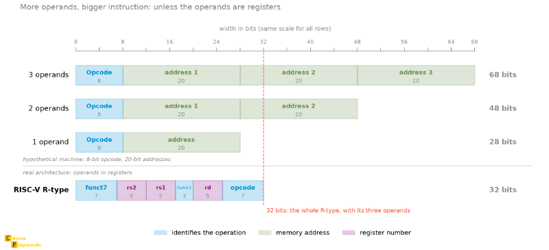
This is the difference that the RISC × CISC discussion usually summarizes poorly: it is not “fewer instructions”, it is operands in registers and a fixed-size format, which together make decoding trivial and the pipeline predictable.
An add rd, rs1, rs2 in RISC-V has opcode = 0110011, funct3 = 000,
and funct7 = 0000000; changing funct7 to 0100000 turns the same
instruction into sub. The operation changes, the format does not, and that
is why the decoder of a RISC processor fits in much less silicon than that of
an x86, where an instruction can have from 1 to 15 bytes.
Strategy for counting the number of instructions
-
3 operands: each operation in the expression generally produces one instruction with an explicit destination. In the expression
\[ X = A \times (B + C \times D - E/F) \]there are 5 arithmetic operations: one multiplication \(C \times D\), one addition, one division, one subtraction, and the final multiplication by \(A\). Therefore, the 3-operand program uses 5 instructions, with no need for an extra “assignment” instruction.
-
2 operands: add
MOVs when you need to preserve a value before overwriting it. -
1 operand: add
LDAandSTRwhenever you need to load data into the accumulator and save intermediate results.
Instructions such as SQRT, NEG, or immediate shifts can appear in real or
hypothetical ISAs, but their presence alone does not define an architecture
as CISC or RISC.
The distinction between RISC and CISC involves a larger set of design decisions:
- regularity of the instruction formats;
- number of addressing modes;
- average complexity of the instructions;
- ease of pipelining and decoding.
Therefore, the following example is just an example of an extended hypothetical ISA, and not a proof of a “CISC philosophy”.
Example: compute \(X_1 = (-B + \sqrt{B^2 - 4C}) / 2\) with 1 operand
Using 1-operand (accumulator) instructions with direct and immediate
addressing, and with the special instruction SQRT for the square root:
The order of operations here requires care. With a single accumulator, \(B^2 - 4C\) cannot be computed in the obvious sequence: subtracting 4 and then multiplying by \(C\) would produce \((B^2 - 4) \times C\), which is a different computation. The way is to compute \(4C\) first, store it in a temporary, and only then subtract:
LDA C        ; ACC = C
MPY #4       ; ACC = 4C            (immediate addressing)
STR TEMP     ; TEMP = 4C
LDA B        ; ACC = B
MPY B        ; ACC = B²
SUB TEMP     ; ACC = B² − 4C
SQRT         ; ACC = √(B² − 4C)
STR TEMP     ; TEMP = √(B² − 4C)   (reuses the temporary)
LDA B        ; ACC = B
NEG          ; ACC = −B
ADD TEMP     ; ACC = −B + √(B² − 4C)
SHR #1       ; ACC = ACC / 2       (shift right = divide by 2)
STR X1       ; X1 = ACC
Thirteen instructions and one temporary address for an expression that, on paper, has five operations. This is the cost of the single accumulator: every intermediate result that cannot be consumed immediately has to be parked in memory.
This formula has a problem that assembly does not solve
The order chosen here is arithmetically correct, but the quadratic formula written this way is numerically unstable in floating point: when \(B^2\) is much larger than \(4C\), the root is almost equal to \(|B|\), and the subtraction of two close numbers destroys the significant digits. This is catastrophic cancellation, discussed in detail in the article on IEEE 754 from the sister series, along with the alternative form that avoids the problem. It is worth mentioning because it is a good example of something this article cannot see: the instruction is right, the encoding is right, and the result can still be wrong, because the representation of numbers is a layer below the representation of instructions.
Addressing modes #
The addressing modes define how the processor obtains the operand of an instruction.
The central point is this: the effective address (EA) is the final address of the operand in memory, when the instruction actually accesses memory. In some modes there is no memory EA, because the data is already in the instruction itself or in a register.
flowchart TD
    A([Instruction]) --> B{Addressing
Mode}
    B --> C["Immediate
operand = constant"]
    B --> D["Direct
EA = address"]
    B --> E["Indirect
EA = M[address]"]
    B --> F["Reg. Direct
operand = Rn"]
    B --> G["Reg. Indirect
EA = Rn"]
    B --> H["Indexed
EA = address + Ri"]
    B --> I["Base + Displacement
EA = RB + disp"]
After computing the EA, when there is a memory access, the operand will be:
$$ \text{Operand} = M[EA] $$For the processor, there are two ways to identify which of these modes to
use: either the Opcode already carries that information (the code 1010
means direct LDA and 1011 means indirect LDA) or the instruction
reserves a specific bit field just to signal the addressing mode to the
decoder.
Immediate mode #
The operand is the constant encoded directly in the instruction: it is not an address, it is the value itself.
$$\text{Operand} = \text{constant in the instruction}$$- Advantage: very fast, with no additional MM access
- Disadvantage: limited by the field size; only serves for small, fixed constants
- Example:
LDA #5→ ACC = 5
Direct (absolute) mode #
The instruction field contains the memory address where the operand is.
$$ EA = \text{address} \qquad\Rightarrow\qquad \text{Operand} = M[EA] $$- Advantage: simple and direct; easy to understand and debug
- Disadvantage: the address is fixed in the object code, which makes relocating the program harder
- Example:
LDA 100→ ACC = M[100]
Indirect mode #
The field contains an address that holds the address of the operand, an extra level of indirection. The field points to a pointer.
$$ EA = M[\text{address}] \qquad\Rightarrow\qquad \text{Operand} = M[EA] $$- Advantage: flexible for pointers and dynamic structures
- Disadvantage: requires 2 MM accesses, one to fetch the address and another to fetch the data
- Example:
LDA @100→ ACC = M[M[100]]
Indirect mode: 2 memory accesses
Indirect mode is often confused with register indirect mode. The difference is in the number of MM accesses:
- Indirect (memory): 2 accesses. The pointer’s address is in memory, so you must fetch the pointer (1st access) and then the data (2nd access)
- Register indirect: 1 access. The pointer is already in a register (no access to fetch it), so there is only the access to the data
Register direct mode #
The operand is in a processor register. Here there is no effective address: there is nothing to compute or to fetch from memory, because the data is already inside the CPU. The operand field in the instruction does not hold an address, it holds the register number:
$$\text{Operand} = R_n \qquad (\text{without } EA)$$-
Advantage: the fastest possible, since reading a register costs about 1 cycle, against 100 to 300 cycles for a main memory access that misses the cache. The difference is two orders of magnitude.
-
Disadvantage: limited number of registers; programs need to manage which data they keep in registers
-
Example:
ADD R1, R2→ R1 = R1 + R2
Register indirect mode #
The register contains the memory address where the operand is. The register works as a pointer.
$$ EA = R_n \qquad\Rightarrow\qquad \text{Operand} = M[EA] $$- Advantage: very flexible for traversing arrays using a register as an incrementable pointer
- Example:
LDA (R1)→ ACC = M[R1]
Indexed mode #
The base address is encoded in the instruction; the index register \(R_i\) is added to it to compute the effective address.
$$ EA = \text{address} + R_i \qquad\Rightarrow\qquad \text{Operand} = M[EA] $$- Advantage: ideal for traversing arrays sequentially, because you just increment \(R_i\) on each iteration
- Example:
LDA 100(R1)→ ACC = M[100 + R1]
Imagine the task of summing 100 numbers in an array. In direct mode, you would have to write the same instruction 100 times, changing only the address. With indexed mode, you write the instruction once, pointing to the base of the array, and use an index register to “walk” through the elements. It is the difference between 300 lines of code and an efficient 5-line loop.
Base + displacement mode #
The register contains the base; the instruction carries a fixed displacement.
$$ EA = R_B + \text{displacement} \qquad\Rightarrow\qquad \text{Operand} = M[EA] $$- Conceptual example: accessing a structure field or a local variable on the stack
- Typical use: relocatable code, stack, function activation, access to struct fields
This mode is very common in modern architectures because it cleanly separates the dynamic base address from the fixed displacement known at compile time.
Modern examples of base + displacement
In current architectures, this mode shows up all the time.
-
x86-64:
mov eax, [rbp-8]Accesses a local variable from the stack base pointer. -
AArch64:
ldr x0, [x1, #16]Accesses the memory location whose address isx1 + 16.
This makes base + displacement mode easier to recognize in real code than old examples based on historical segmentation.
Indexed × base + displacement
In both cases, the final address is the sum of two values. The difference is:
-
Indexed: base in the instruction + index in the register Ideal for arrays and iteration.
-
Base + displacement: base in the register + displacement in the instruction Ideal for the stack, structs, and relocatable code.
Comparison table #
| Mode | EA | Operand | MM accesses to get the data | Main advantage |
|---|---|---|---|---|
| Immediate | (none) | value in the instruction | 0 | Constants; maximum speed |
| Direct | \(\text{address}\) | \(M[EA]\) | 1 | Simple; global variables |
| Indirect | \(M[\text{address}]\) | \(M[EA]\) | 2 | Pointers in memory |
| Reg. Direct | (none) | \(R_n\) | 0 | Fast operation on registers |
| Reg. Indirect | \(R_n\) | \(M[EA]\) | 1 | Pointer in a register |
| Indexed | \(\text{address} + R_i\) | \(M[EA]\) | 1 | Traversing arrays |
| Base + Displacement | \(R_B + \text{disp}\) | \(M[EA]\) | 1 | Stack, structs, relocation |
Example: addressing modes with a memory table
Consider the memory:
| Address | Contents |
|---|---|
| 1AC1 | 1AC6 |
| 1AC2 | 1AC4 |
| 1AC3 | 1AC1 |
| 1AC4 | 1AC3 |
| 1AC5 | 1AC1 |
| 1AC6 | 1AC5 |
a) Direct, operand = 1AC1
$$ EA = 1AC1 \qquad\Rightarrow\qquad ACC \leftarrow M[1AC1] = \mathbf{1AC6} $$b) Immediate, operand = 1AC5
The operand field already contains the value:
$$ ACC \leftarrow \mathbf{1AC5} $$c) Indirect, operand = 1AC3
First the effective address is computed:
$$ EA = M[1AC3] = 1AC1 $$Then the operand is fetched:
$$ ACC \leftarrow M[EA] = M[1AC1] = \mathbf{1AC6} $$d) If the contents of 1AC1 change to 0
- Direct: \(ACC = M[1AC1] = \mathbf{0}\)
- Immediate: \(ACC = \mathbf{1AC5}\) (unchanged)
- Indirect: \(EA = M[1AC3] = 1AC1 \Rightarrow ACC = M[1AC1] = \mathbf{0}\)
Immediate mode is the only one that does not depend on the current contents of memory.
Python bonus: computing effective addresses #
Understanding hardware by reading diagrams and mathematical formulas can seem very abstract at first. But, in the end, addressing modes are just pointer calculation logic. For a programmer, the easiest way to demystify what the silicon does is to translate that mechanics into code. See how the hardware would compute effective addresses using simple Python functions:
# Simulates the main addressing modes.
# Mind the convention: each function returns the OPERAND (the data the
# instruction wanted) and the number of MM accesses that were needed, not
# the effective address. The EA shows up along the way, commented where
# relevant.

def ea_immediate(value):
    """Immediate mode: the operand is the value itself."""
    return value, 0  # (data, MM accesses)


def ea_direct(memory: dict, address: int):
    """Direct mode: EA = address; operand = M[EA]."""
    return memory[address], 1


def ea_indirect(memory: dict, address: int):
    """Indirect mode: EA = M[address]; operand = M[EA]."""
    ptr = memory[address]            # 1st access: fetches the pointer (= EA)
    return memory[ptr], 2            # 2nd access: fetches the data


def ea_reg_indirect(memory: dict, register: int):
    """Register indirect mode: EA = Rn; operand = M[EA].

    The parameter receives the CONTENTS of the register, which is already
    the address.
    """
    return memory[register], 1


def ea_indexed(memory: dict, base: int, index: int):
    """Indexed mode: EA = base + Ri; operand = M[EA]."""
    return memory[base + index], 1


def ea_base_displacement(memory: dict, rb: int, displacement: int):
    """Base + displacement mode: EA = RB + displacement; operand = M[EA]."""
    return memory[rb + displacement], 1


# Memory table from the previous example
mem = {
    0x1AC1: 0x1AC6,
    0x1AC2: 0x1AC4,
    0x1AC3: 0x1AC1,
    0x1AC4: 0x1AC3,
    0x1AC5: 0x1AC1,
    0x1AC6: 0x1AC5,
}

data, accesses = ea_direct(mem, 0x1AC1)
print(f"Direct   (1AC1): {data:04X}  ({accesses} MM access(es))")
# Direct   (1AC1): 1AC6  (1 MM access(es))

data, accesses = ea_immediate(0x1AC5)
print(f"Immediate(1AC5): {data:04X}  ({accesses} MM access(es))")
# Immediate(1AC5): 1AC5  (0 MM access(es))

data, accesses = ea_indirect(mem, 0x1AC3)
print(f"Indirect (1AC3): {data:04X}  ({accesses} MM access(es))")
# Indirect (1AC3): 1AC6  (2 MM access(es))

# Array with indexed mode
array = {100: 10, 101: 20, 102: 30, 103: 40}
for i in range(4):
    val, _ = ea_indexed(array, 100, i)
    print(f"array[{i}] = {val}")
# array[0] = 10, array[1] = 20, array[2] = 30, array[3] = 40
Conclusion and next articles #
The ISA defines the vocabulary the processor understands; instruction formats and addressing modes are the grammar of that vocabulary. With three operands per instruction and seven addressing modes, a processor can express anything from simple additions to dynamic access to complex data structures. The choice between more operands (CISC) and fewer operands (RISC) reflects a trade-off between expressiveness and regularity that modern hardware resolves in sophisticated ways, the topic of the article Advanced Architectures, at the end of the series.
If you want to see real instructions being generated right now, the Compiler Explorer is the right tool: you write C, C++, Rust, or a dozen other languages on one side and see, on the other, the assembly the compiler produces, and you can choose the architecture, including RISC-V, and compare the formats this article described. It is the fastest way to get out of the table and down to the bit.
In the next article, we will follow the life cycle of a program: from source code in a high-level language, through compilation, linking, and loading, until it becomes the machine instructions the processor executes. We will see how the ISA is the bridge between the code we write and the silicon that executes it, and how ISA design decisions impact the efficiency and flexibility of programs.
See you then!


