

You invest \(1000\) reais at \(1\%\) per month: next month you have \(1010\), then \(1020.10\), then \(1030.30\ldots\) On the other side, anyone who finances a car knows that this month’s outstanding balance is last month’s balance minus the payment, plus interest on what is still owed. In both cases, computing the value for month 12 requires knowing the one for month 11: there is no direct shortcut. Sequences like these, where each term depends on the previous ones, are called recurrence relations.
But the concept goes beyond finance. How many moves are needed to solve the Tower of Hanoi with \(n\) disks? A simple equation, \(T_n = 2T_{n-1} + 1\), contains the complete answer. That is the power of recurrence relations: describing an entire sequence from a local rule.
In this article we define the concept formally, see classic examples and learn the substitution method to obtain closed-form formulas, direct expressions that compute the \(n\)-th term without depending on the previous ones. At the end, we also see the characteristic equation, a technique that extends the repertoire to order-2 recurrences, and divide-and-conquer recurrences, with the Master Theorem.
Why Recurrence Relations? #
Sequences defined in terms of themselves appear throughout computer science and discrete mathematics:
- Analysis of recursive algorithms: the complexity of merge sort, quicksort and the Tower of Hanoi is naturally expressed by recurrences; solving them gives the algorithm’s \(O\) notation (see Divide-and-Conquer Recurrences).
- Combinatorial counting: the number of paths on a grid, triangulations of polygons and integer partitions satisfy recurrences that let us compute large terms from small ones.
- Growth modeling: rabbit populations (Fibonacci), growth with compound interest and basic epidemiological models are all recurrence relations.
- Dynamic programming: a technique for recurrences whose subproblems repeat. Each result is stored so it is not recomputed, and the cost becomes proportional to the number of distinct subproblems. In optimization problems, it also depends on the optimal solution being built from optimal solutions to the subproblems (optimal substructure).
- Formal languages and compilers: context-free grammars generate languages whose number of derivations satisfies recurrences; analyzing their complexity uses the same tools as this article.
What Is a Recurrence Relation? #
A recurrence relation is a formula that relates a term \(a_n\) to some of its predecessors \(a_{n-1}, a_{n-2}, \ldots\). Also called a difference equation. More at Recurrence relation.
To determine the sequence completely, we need the initial conditions, the values of \(a_1, a_2, \ldots\) that serve as the starting point.
A simple example: the partial sums \(S_n = 1 + 2 + \cdots + n\) satisfy
$$S_n = S_{n-1} + n, \quad S_1 = 1$$At each step, we just add \(n\) to the previous value.
Example: Valid Arithmetic Expressions #
Consider expressions formed by digits (\(0{-}9\)) and arithmetic symbols
(\(+,-,\times,\div\)), obeying two rules: the expression must begin and end
with a digit, and two symbols cannot appear consecutively. We call such a
sequence “valid” in the syntactic sense: the rules check only the structure of
the string, not the mathematical meaning. So 5÷0 is counted as valid (it obeys
both rules), even though division by zero is undefined.
For example:
| Expression | Valid? | Reason |
|---|---|---|
0187 |
✓ | digits only |
1+99 |
✓ | begins and ends with a digit, no consecutive symbols |
5×3– |
✗ | ends with a symbol |
6÷+2 |
✗ | two consecutive symbols (\(\div\) and \(+\)) |
Let \(N_k\) be the number of valid expressions of length \(k\).
Initial conditions: \(N_0 = 0\), \(N_1 = 10\) (the digits \(0{-}9\))
Building the recurrence:
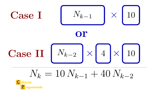
To obtain an expression of length \(k\) from shorter ones, there are two strategies:
- Append a digit (10 options) to the right of an expression of length \(k-1\): contribution \(10 N_{k-1}\)
- Append a symbol + digit (\(4 \times 10 = 40\) options) to the right of an expression of length \(k-2\): contribution \(40 N_{k-2}\)
The following diagram summarizes the two strategies and the resulting formula:
Checking for \(k = 3\)
We want to count expressions of length 3. The two strategies produce:
Strategy 1: append a digit to an expression of length 2
(\(N_2 = 100\) expressions, such as 01, 19, 53…):
Generated examples: 017, 195, 530…
Strategy 2: append a symbol + digit to an expression of length 1 (\(N_1 = 10\) expressions, the digits \(0{-}9\)):
$$40 \times N_1 = 40 \times 10 = 400$$Generated examples: 1+9, 5×3, 0÷7…
Total: \(N_3 = 1{,}000 + 400 = 1{,}400\) ✓
Computing the first terms:
| \(k\) | \(N_k\) |
|---|---|
| 0 | 0 |
| 1 | 10 |
| 2 | 100 |
| 3 | 1,400 |
| 4 | 18,000 |
In \(N_k = 10N_{k-1} + 40N_{k-2}\), each term depends on the two previous terms. We call this an order-2 recurrence. The examples that follow (Tower of Hanoi and others) depend only on the immediately preceding term (order 1), and that is the case where the substitution method presented in this article works well. For order-2 recurrences there is a specific technique, the characteristic equation, presented at the end of this article.
The Fibonacci Sequence: The Rabbit Problem #
The classic Fibonacci problem (1202): a colony of rabbits grows according to these rules:
- It starts with 1 newborn pair
- Every pair that is at least 2 months old produces 1 new pair per month
- No rabbit dies
Let \(F_n\) be the number of pairs at the end of month \(n\). The pairs in month \(n\) are:
- Those that existed in the previous month (\(F_{n-1}\) pairs)
- Those newly born this month, which correspond to the pairs that were at least 2 months old in the previous month (\(F_{n-2}\) pairs)
| \(n\) | 1 | 2 | 3 | 4 | 5 | 6 | 7 | 8 | 9 | 10 | 11 | 12 | 13 |
|---|---|---|---|---|---|---|---|---|---|---|---|---|---|
| \(F_n\) | 1 | 1 | 2 | 3 | 5 | 8 | 13 | 21 | 34 | 55 | 89 | 144 | 233 |
At the end of 13 months: 233 pairs.
The family tree below shows how each adult pair produces a new pair every month, making it visible why \(F_n = F_{n-1} + F_{n-2}\):
flowchart TD
  subgraph m1 ["Month 1: F₁ = 1"]
    A["pair A (newborn)"]
  end
  subgraph m2 ["Month 2: F₂ = 1"]
    B["pair A (adult)"]
  end
  subgraph m3 ["Month 3: F₃ = 2"]
    C["pair A"]
    D["pair B (newborn)"]
  end
  subgraph m4 ["Month 4: F₄ = 3"]
    E["pair A"]
    F["pair B (adult)"]
    G["pair C (newborn)"]
  end
  subgraph m5 ["Month 5: F₅ = 5"]
    H["pair A"]
    I["pair B"]
    J["pair C (adult)"]
    K["pair D (newborn)"]
    L["pair E (newborn)"]
  end
  A --> B
  B --> C
  B -->|produces| D
  C --> E
  D --> F
  C -->|produces| G
  E --> H
  F --> I
  G --> J
  E -->|produces| K
  F -->|produces| L
Tower of Hanoi #
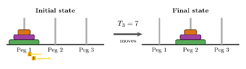
The Tower of Hanoi puzzle was proposed by Édouard Lucas in 1883. We are given \(n\) disks of different sizes stacked in decreasing order on one peg. The goal is to transfer all of them to another peg, using an auxiliary peg, obeying:
- Move only one disk at a time (always from the top)
- Never place a larger disk on top of a smaller one
Let \(T_n\) be the minimum number of moves for \(n\) disks.
The figure below shows the initial state (all disks on Peg 1) and the desired final state (all on Peg 2) for \(n = 3\):
A concrete example: n = 3
Before thinking about formulas, let’s see what happens step by step with 3 disks. Each arrow in the figure below represents a single move: always the top disk of one peg to the top of another, respecting the rule of never placing a larger disk on a smaller one. Read the top row from left to right (States 0 → 3), go down to State 4, and read the bottom row from right to left (States 4 → 7):
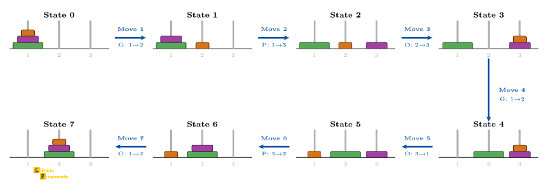
Exactly 7 moves were needed to transfer the 3 disks. To try other numbers of disks, there are interactive simulators, such as the one at Math is Fun.
Finding the recursive pattern
Looking closely at the 7 moves, we notice a structure in three blocks:
- Moves 1 to 3 (States 0 → 3): the 2 smaller disks go from Peg 1 to Peg 3, using Peg 2 as the auxiliary, in exactly \(T_2 = 3\) moves.
- Move 4 (State 3 → 4): the largest disk goes alone from Peg 1 to Peg 2, in 1 move.
- Moves 5 to 7 (States 4 → 7): the 2 smaller disks go from Peg 3 to Peg 2, using Peg 1 as the auxiliary, again \(T_2 = 3\) moves.
Total: \(T_3 = 3 + 1 + 3 = 7\). ✓
The same reasoning applies to any \(n\): to move \(n\) disks, we always need to (1) solve the problem of size \(n-1\), (2) move the largest disk, and (3) solve the problem of size \(n-1\) again. The diagram below summarizes this recursive algorithm. Each block labeled \(T_{n-1}\) represents a complete subproblem with many individual moves, not a single step:
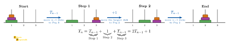
Why can’t it be done with fewer? The construction above shows that \(2T_{n-1} + 1\) moves are sufficient. They are also necessary, because the largest disk must leave the source peg at least once:
- At the first move of the largest disk, the other \(n-1\) disks are all on the third peg: they cannot be on the largest disk’s peg, nor on the peg it is going to. Getting them there took at least \(T_{n-1}\) moves.
- At the last move of the largest disk, which leaves it at the destination, the other \(n-1\) are also all on a single peg, which is not the destination. Stacking them on top of the largest requires at least another \(T_{n-1}\) moves.
Adding the largest disk’s own move, no solution takes fewer than \(2T_{n-1} + 1\) moves. With both bounds together, we formalize:
$$T_n = 2T_{n-1} + 1, \quad T_1 = 1$$Computing the first values:
| \(n\) | 1 | 2 | 3 | 4 |
|---|---|---|---|---|
| \(T_n\) | 1 | 3 | 7 | 15 |
The call tree of \(T(3)\) makes the recurrence visible. Each node \(T(k)\) unfolds into two children \(T(k-1)\) plus one unit, until it reaches the base case \(T(1) = 1\):
flowchart TD
  T3["T(3) = 7"]
  T2a["T(2) = 3"]
  M1["+1"]
  T2b["T(2) = 3"]
  T1a["T(1) = 1"]
  M2["+1"]
  T1b["T(1) = 1"]
  T1c["T(1) = 1"]
  M3["+1"]
  T1d["T(1) = 1"]
  T3 --> T2a & M1 & T2b
  T2a --> T1a & M2 & T1b
  T2b --> T1c & M3 & T1d
The Substitution Method #
The substitution method consists of applying the recurrence relation repeatedly, replacing each term by its own recurrence, until a general pattern emerges.
Every application of the method follows the same five steps:
| Step | What to do |
|---|---|
| 1. Write the recurrence | Express \(T(n)\) in terms of \(T(n-1)\) (or \(T(n-2)\), etc.) with an initial condition |
| 2. Substitute iteratively | Replace \(T(n-1)\) by its own recurrence, then \(T(n-2)\), and so on |
| 3. Recognize the pattern | Generalize the expression for \(T(n)\) in terms of \(T(n-k)\) and the accumulated constants |
| 4. Use the initial condition | When \(k = n-1\) (or equivalent), substitute the base case to eliminate \(T\) |
| 5. Verify by induction | Prove that the formula obtained is correct for all \(n\) using mathematical induction |
The diagram below summarizes the flow of the method:
flowchart LR
  E1["1. Write
the recurrence"] --> E2["2. Substitute
iteratively"]
  E2 --> E3["3. Recognize
the pattern"]
  E3 --> E4["4. Use the
initial condition"]
  E4 --> E5["5. Verify
by induction"]
  E5 --> FEC(["closed-form formula ✓"])
Solving the Tower of Hanoi #
$$T_n = 2T_{n-1} + 1$$Substituting iteratively:
$$T_n = 2T_{n-1} + 1 = 2(2T_{n-2}+1)+1 = 2^2 T_{n-2} + 2 + 1$$$$= 2^2(2T_{n-3}+1)+2+1 = 2^3 T_{n-3} + 2^2 + 2 + 1 = \cdots$$$$= 2^{n-1} T_1 + 2^{n-2} + \cdots + 2 + 1 = 2^{n-1} + \sum_{k=0}^{n-2} 2^k = 2^{n-1} + (2^{n-1} - 1) = 2^n - 1$$Closed-form formula: \(T_n = 2^n - 1\)
Verification by induction:
Base case (\(n=1\)): \(T_1 = 1 = 2^1 - 1\) ✓
IH: \(T_k = 2^k - 1\)
Inductive step (\(n = k+1\)):
$$T_{k+1} = 2T_k + 1 \stackrel{\text{IH}}{=} 2(2^k - 1) + 1 = 2^{k+1} - 2 + 1 = 2^{k+1} - 1$$Therefore, \(T_n = 2^n - 1\), which is what we wanted to prove. \(\blacksquare\)
Lucas proposed the problem with 64 disks, claiming that the end of the world would occur when the Brahmins of a temple in Benares finished moving them. With the formula: \(T_{64} = 2^{64} - 1 \approx 1.8 \times 10^{19}\) moves. Even at 1 move per second, it would take more than 580 billion years.
Édouard Lucas also gives his name to the Lucas sequence (2, 1, 3, 4, 7, 11, 18, …), which follows the same rule as Fibonacci, \(L_n = L_{n-1} + L_{n-2}\), with other initial conditions (\(L_0 = 2\), \(L_1 = 1\)). And to the Lucas-Lehmer test, created by him in 1878 and proved by Derrick Lehmer in 1930: a primality test for Mersenne numbers \(2^p - 1\) that is faster than general tests. That is why many of the largest known primes are Mersenne primes.
Application: Tower of Hanoi in Python
The recursive solution directly implements the three steps of the algorithm:
def hanoi(n, source="A", destination="C", auxiliary="B"):
    if n == 1:
        print(f"Move disk 1: {source} → {destination}")
        return 1
    total  = hanoi(n - 1, source, auxiliary, destination)
    print(f"Move disk {n}: {source} → {destination}")
    total += 1 + hanoi(n - 1, auxiliary, destination, source)
    return total

print(hanoi(3))  # prints the 7 moves and returns 7
The proof by induction validates the code step by step:
| Step | In the proof | In the code |
|---|---|---|
| Base case | \(T_1 = 1\) | if n == 1: return 1: 1 disk, 1 move |
| IH | \(T_k = 2^k - 1\) moves | hanoi(n-1, ...) returns the correct value (by hypothesis) |
| Inductive step | \(T_n = 2T_{n-1} + 1\) | total = hanoi(n-1,...) + 1 + hanoi(n-1,...) |
Calling hanoi(64) would take the same astronomical time computed above, and
there is no shortcut: the minimality argument, made before the recurrence,
shows that \(2^n - 1\) moves is the minimum possible for any algorithm, not
just this one.
Example: Ovals in the Plane #
We are given \(n\) ovals in the plane obeying two conditions:
- Any two ovals cross at exactly 2 distinct points
- No point belongs to three or more ovals simultaneously (no triple point)
Into how many regions do these \(n\) ovals divide the plane?
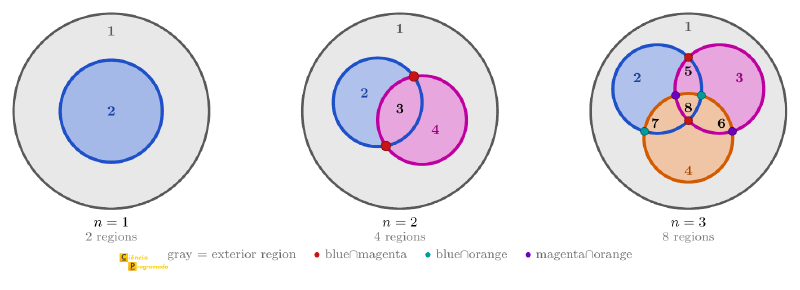
The figure below shows the cases \(n = 1, 2, 3\) with numbered regions and marked intersection points (colored dots = intersections between pairs of ovals):
Looking at the concrete cases:
| \(k\) | Previous ovals | Intersections with the previous ones | New arcs | New regions | Total \(a_k\) |
|---|---|---|---|---|---|
| 1 | 0 | n/a | n/a | n/a | 2 (base) |
| 2 | 1 | 2 points | 2 arcs | 2 | 4 |
| 3 | 2 | 4 points | 4 arcs | 4 | 8 |
| 4 | 3 | 6 points | 6 arcs | 6 | 14 |
Why does each new oval add exactly \(2(k-1)\) regions?
When the \(k\)-th oval enters the plane, it crosses each of the \(k-1\) previous ovals at exactly 2 points, creating \(2(k-1)\) intersection points on it. These points divide the boundary of the new oval into \(2(k-1)\) stretches of curve (called arcs): each one is the segment of the boundary between two consecutive intersection points.
The key is that each arc lies entirely within a single existing region (since the existing boundaries are crossed only at the intersection points). By crossing that region, the arc divides it in two, creating exactly 1 new region per arc.
A concrete example (\(k = 3\), the orange oval in the \(n=3\) panel): The orange oval crosses the blue oval at 2 points (green dots) and the magenta oval at 2 points (violet dots), 4 points in total, which divide the orange boundary into 4 arcs. Each arc cuts one of the 4 existing regions in half: \(4 + 4 = 8\) regions. ✓
Let \(a_k\) be the number of regions with \(k\) ovals:
$$a_k = a_{k-1} + 2(k-1), \quad a_1 = 2$$Solving by substitution:
$$a_n = 2 + \sum_{k=2}^{n} 2(k-1) = 2 + 2\sum_{j=1}^{n-1} j = 2 + 2 \cdot \frac{(n-1)n}{2} = 2 + n(n-1)$$Closed-form formula: \(a_n = n^2 - n + 2\)
Checking: \(a_1 = 1 - 1 + 2 = 2\) ✓, \(a_2 = 4 - 2 + 2 = 4\) ✓, \(a_3 = 9 - 3 + 2 = 8\) ✓, \(a_4 = 16 - 4 + 2 = 14\) ✓
Going Further: Order-2 Recurrences #
The substitution method solves recurrences where each term depends only on the previous one. For linear homogeneous recurrences of order 2 (those in which each term is a linear combination of the two previous ones, with no independent terms) there is a systematic technique called the characteristic equation: we assume the solution has the form \(a_n = r^n\) and find which values of \(r\) satisfy the recurrence. The pipeline below summarizes the complete flow for the case of distinct roots (\(\Delta \neq 0\)):
flowchart LR
  R["linear homogeneous
recurrence of order 2"] --> S["assume
aₙ = rⁿ"]
  S --> Q["characteristic
equation"]
  Q --> Ro["distinct roots
r₁ ≠ r₂"]
  Ro --> G["general solution
A·r₁ⁿ + B·r₂ⁿ"]
  G --> CI["initial
conditions"]
  CI --> FC(["closed-form formula ✓"])
For repeated roots (\(\Delta = 0\)), the correct form is \((A + Bn) \cdot r^n\); this case does not occur in the examples of this article.
Fibonacci #
The recurrence \(F_n = F_{n-1} + F_{n-2}\) with \(F_1 = F_2 = 1\).
Substituting \(F_n = r^n\) into the recurrence:
$$r^n = r^{n-1} + r^{n-2}$$Dividing both sides by \(r^{n-2}\) (with \(r \neq 0\)):
$$r^2 = r + 1 \implies r^2 - r - 1 = 0$$By the quadratic formula:
$$r = \frac{1 \pm \sqrt{1 + 4}}{2} = \frac{1 \pm \sqrt{5}}{2}$$The two roots are \(\varphi = \dfrac{1+\sqrt{5}}{2} \approx 1.618\) (the golden ratio) and \(\psi = \dfrac{1-\sqrt{5}}{2} \approx {-0.618}\). Since both are independent solutions, the general solution is any linear combination of them:
$$F_n = A \varphi^n + B \psi^n$$Using \(F_1 = 1\) and \(F_2 = 1\) to determine \(A\) and \(B\):
Step 1: subtract the equations from the initial conditions:
$$F_2 - F_1 = A(\varphi^2 - \varphi) + B(\psi^2 - \psi) = 0$$Since \(\varphi^2 - \varphi = \varphi(\varphi - 1) = 1\) and \(\psi^2 - \psi = 1\) (both roots satisfy \(r^2 = r+1\)), this gives \(A + B = 0\), hence \(B = -A\).
Step 2: substitute \(B = -A\) into \(F_1 = 1\):
$$A(\varphi - \psi) = 1 \implies A = \frac{1}{\varphi - \psi} = \frac{1}{\sqrt{5}}$$We obtain Binet’s formula:
$$F_n = \frac{\varphi^n - \psi^n}{\sqrt{5}}$$The previous article in the series proves this formula by strong induction.
Arithmetic Expressions #
The recurrence \(N_k = 10N_{k-1} + 40N_{k-2}\) with \(N_0 = 0\) and \(N_1 = 10\).
Substituting \(N_k = r^k\) and dividing by \(r^{k-2}\):
$$r^2 - 10r - 40 = 0 \implies r = \frac{10 \pm \sqrt{100 + 160}}{2} = 5 \pm \sqrt{65}$$The general solution is \(N_k = A(5+\sqrt{65})^k + B(5-\sqrt{65})^k\). Using the initial conditions:
- \(N_0 = 0 \implies A + B = 0 \implies B = -A\)
- \(N_1 = 10 \implies A \cdot 2\sqrt{65} = 10 \implies A = \dfrac{\sqrt{65}}{13}\)
Closed-form formula:
$$N_k = \frac{\sqrt{65}}{13}\left[\left(5+\sqrt{65}\right)^k - \left(5-\sqrt{65}\right)^k\right]$$Checking against the table:
- \(N_1 = \dfrac{\sqrt{65}}{13} \cdot 2\sqrt{65} = \dfrac{130}{13} = 10\) ✓
- \(N_2 = \dfrac{\sqrt{65}}{13} \cdot 20\sqrt{65} = \dfrac{1300}{13} = 100\) ✓
The contrast with Fibonacci is instructive: the same technique produces results of very different elegance. Closed-form formulas always exist for linear recurrences with constant coefficients, written from the roots of the characteristic equation, but they are not always pretty.
Divide-and-Conquer Recurrences #
All the recurrences so far step back one or two terms: \(T_{n-1}\), \(T_{n-2}\). Divide-and-conquer algorithms do something else: they break the input into parts that are a fraction of the original size. Merge sort, seen in the article on strong induction, splits the list in half, sorts each half and merges the two sorted halves in time proportional to \(n\). Counting the cost \(T(n)\) for \(n\) elements:
$$T(n) = 2T(n/2) + n, \quad T(1) = 1$$To keep the calculations exact, we take \(n\) to be a power of 2; for other values of \(n\), the roundings of \(n/2\) change the constants, but not the growth.
Solving by substitution #
With \(n = 2^m\), the recurrence steps back through the powers of 2 and the substitution method works as before:
$$T(n) = 2T(n/2) + n = 2\left[2T(n/4) + \frac{n}{2}\right] + n = 4T(n/4) + 2n$$$$= 4\left[2T(n/8) + \frac{n}{4}\right] + 2n = 8T(n/8) + 3n = \cdots = 2^i T(n/2^i) + i \cdot n$$The substitution stops at \(i = m = \log_2 n\), when \(n/2^m = 1\):
$$T(n) = 2^m T(1) + m \cdot n = n + n \log_2 n$$Closed-form formula: \(T(n) = n \log_2 n + n\); therefore, \(T(n) = O(n \log n)\), as announced in the series introduction article.
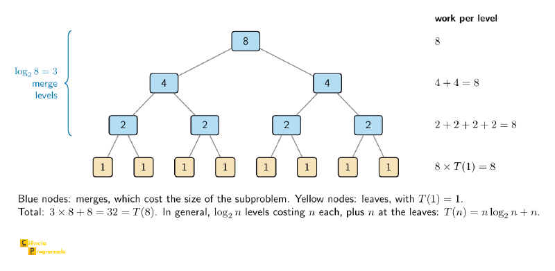
The recursion tree shows where each term comes from. In the figure below, for \(n = 8\), each level doubles the number of subproblems and halves the size of each one, so the merges at each level always add up to 8; there are \(\log_2 8 = 3\) levels of merging, and the 8 leaves add another 8:
Verification by induction (on \(m\), with \(n = 2^m\)):
Base case (\(m = 0\), \(n = 1\)): \(T(1) = 1 = 1 \cdot 0 + 1\) ✓
IH: \(T(2^k) = 2^k \cdot k + 2^k\)
Inductive step (\(m = k+1\)):
$$T(2^{k+1}) = 2T(2^k) + 2^{k+1} \stackrel{\text{IH}}{=} 2\left(2^k k + 2^k\right) + 2^{k+1} = 2^{k+1}(k+1) + 2^{k+1}$$Therefore, \(T(n) = n \log_2 n + n\) for every power of 2, \(n = 2^m\), which is what we wanted to prove. \(\blacksquare\)
The Master Theorem #
The same reasoning holds for any algorithm that splits the input into \(a\) subproblems of size \(n/b\) and spends extra work of the order of \(n^d\) to divide and combine. The result is the Master Theorem, here in its most commonly used form:
If \(T(n) = aT(n/b) + \Theta(n^d)\), with constants \(a \geq 1\), \(b > 1\) and \(d \geq 0\), then:
- \(T(n) = \Theta(n^d)\), if \(d > \log_b a\);
- \(T(n) = \Theta(n^d \log n)\), if \(d = \log_b a\);
- \(T(n) = \Theta(n^{\log_b a})\), if \(d < \log_b a\).
The \(\Theta\) notation indicates exact growth: the function stays between two constant multiples of \(n^d\) (or of whatever is inside the \(\Theta\)), above and below.
The intuition comes from the recursion tree. At each level, the number of subproblems is multiplied by \(a\) and the work of each one by \(1/b^d\), that is, the total work of the level is multiplied by \(a/b^d\). If \(a/b^d < 1\) (that is, \(d > \log_b a\)), the work shrinks at each level and the root dominates. If \(a/b^d = 1\), all \(\log_b n\) levels cost the same. If \(a/b^d > 1\), the work grows at each level and the \(n^{\log_b a}\) leaves dominate.
| Algorithm | Recurrence | \(a\), \(b\), \(d\) | Case | Result |
|---|---|---|---|---|
| Merge sort | \(T(n) = 2T(n/2) + \Theta(n)\) | 2, 2, 1 | \(d = \log_2 2 = 1\) | \(\Theta(n \log n)\) |
| Binary search | \(T(n) = T(n/2) + \Theta(1)\) | 1, 2, 0 | \(d = \log_2 1 = 0\) | \(\Theta(\log n)\) |
| Karatsuba multiplication | \(T(n) = 3T(n/2) + \Theta(n)\) | 3, 2, 1 | \(d < \log_2 3 \approx 1.58\) | \(\Theta(n^{\log_2 3})\) |
| Quadratic merge (hypothetical) | \(T(n) = 2T(n/2) + \Theta(n^2)\) | 2, 2, 2 | \(d > \log_2 2 = 1\) | \(\Theta(n^2)\) |
Binary search discards half of the interval at each step and spends constant time deciding which half stays. Karatsuba’s algorithm multiplies two numbers of \(n\) digits with three multiplications of numbers of \(n/2\) digits, instead of the four of the grade-school method. The last row shows what would happen with a merge sort whose merge was quadratic: the work at the root would come to dominate.
The simplified form requires subproblems of the same size \(n/b\) and extra work of the form \(n^d\). Recurrences such as \(T(n) = T(n-1) + n\) (which steps back one term, not a fraction) or \(T(n) = 2T(n/2) + n \log n\) are left out: the first is solved by substitution, as at the beginning of this article, and the second needs the general form of the theorem, described in the entry cited above.
Checking the formulas in Python
Every closed-form formula in this article can be checked by iterating the recurrence and comparing the terms:
from math import isclose, sqrt

# Tower of Hanoi: T1 = 1, Tn = 2 T(n-1) + 1
T = {1: 1}
for n in range(2, 31):
    T[n] = 2 * T[n - 1] + 1
print(all(T[n] == 2**n - 1 for n in T))  # True

# Ovals in the plane: a1 = 2, an = a(n-1) + 2(n-1)
a = {1: 2}
for n in range(2, 31):
    a[n] = a[n - 1] + 2 * (n - 1)
print(all(a[n] == n**2 - n + 2 for n in a))  # True

# Arithmetic expressions: N0 = 0, N1 = 10, Nk = 10 N(k-1) + 40 N(k-2)
N = {0: 0, 1: 10}
for k in range(2, 21):
    N[k] = 10 * N[k - 1] + 40 * N[k - 2]
r1, r2 = 5 + sqrt(65), 5 - sqrt(65)
print(all(isclose(N[k], sqrt(65) / 13 * (r1**k - r2**k)) for k in N))  # True

# Merge sort, with n = 2^m: T(1) = 1, T(n) = 2 T(n/2) + n
M = {0: 1}
for m in range(1, 31):
    M[m] = 2 * M[m - 1] + 2**m
print(all(M[m] == 2**m * m + 2**m for m in M))  # True
The comparison with isclose for the arithmetic expressions is necessary
because the closed-form formula involves \(\sqrt{65}\), which the computer
stores only approximately.
Summary Table #
The results proved in this article, gathered for quick reference:
| Sequence | Base | Recurrence | Closed-Form Formula |
|---|---|---|---|
| Fibonacci | \(F_1 = F_2 = 1\) | \(F_n = F_{n-1} + F_{n-2}\) | \(F_n = \dfrac{\varphi^n - \psi^n}{\sqrt{5}}\) (Binet) |
| Tower of Hanoi | \(T_1 = 1\) | \(T_n = 2T_{n-1} + 1\) | \(T_n = 2^n - 1\) |
| Ovals in the plane | \(a_1 = 2\) | \(a_n = a_{n-1} + 2(n-1)\) | \(a_n = n^2 - n + 2\) |
| Partial sums | \(S_1 = 1\) | \(S_n = S_{n-1} + n\) | \(S_n = n(n+1)/2\) |
| Arithmetic expressions | \(N_0 = 0,\ N_1 = 10\) | \(N_k = 10N_{k-1} + 40N_{k-2}\) | \(N_k = \dfrac{\sqrt{65}}{13}\left[(5+\sqrt{65})^k - (5-\sqrt{65})^k\right]\) |
| Merge sort (\(n = 2^m\)) | \(T(1) = 1\) | \(T(n) = 2T(n/2) + n\) | \(T(n) = n \log_2 n + n\) |
Exercises #
Practice setting up and solving recurrences with the substitution method. Exercises 1 and 2 follow the model of the examples seen; exercises 3 and 4 demand more attention to setting up the recurrence and to the algebraic verification.
Exercise 1: Double Tower of Hanoi
A variant of Hanoi: \(2n\) disks of \(n\) sizes, two of each size. The rules are the same as in the classic Hanoi.
(a) Set up the recurrence relation. (b) Solve it by the substitution method.
Solutions
(a) To move \(2n\) disks: move the \(2(n-1)\) smallest (\(T(n-1)\) moves), move the 2 largest (2 moves), move the \(2(n-1)\) smallest back (\(T(n-1)\) moves).
$$T(1) = 2, \quad T(n) = 2T(n-1) + 2 \text{ for } n \geq 2$$(b) By iterative substitution:
$$T(n) = 2T(n-1) + 2 = 2^i T(n-i) + \sum_{k=1}^i 2^k$$For \(i = n-1\):
$$T(n) = 2^{n-1} \cdot T(1) + \sum_{k=1}^{n-1} 2^k = 2^n + (2^n - 2) = \mathbf{2^{n+1} - 2}$$
Exercise 2: Unbounded regions formed by lines
Let \(a_n\) be the number of unbounded regions created by \(n\) lines in general position (no parallels and no triple point).
(a) Illustrate for \(n = 0, 1, 2, 3, 4\). (b) Set up and solve the recurrence.
Solutions
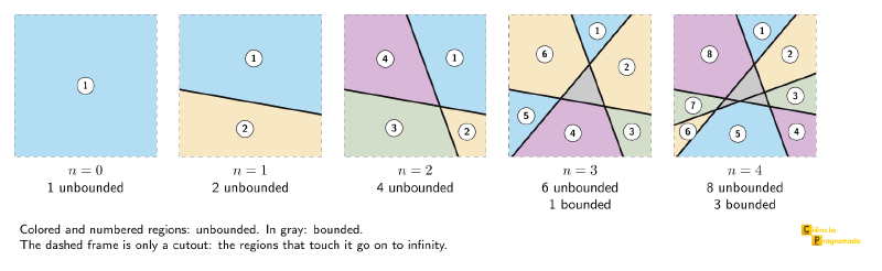
(a) From the second line on, each new line adds 2 unbounded regions, one at each end. The first is an exception, because it divides the whole plane (1 region) into two half-planes, an increase of only 1 region:
| \(n\) | \(a_n\) |
|---|---|
| 0 | 1 |
| 1 | 2 |
| 2 | 4 |
| 3 | 6 |
| 4 | 8 |
The figure below illustrates the five cases, with the unbounded regions numbered around the frame and the bounded ones in gray, which do not count:
(b) \(a_n = a_{n-1} + 2\) for \(n \geq 2\), with \(a_1 = 2\). The case \(a_0 = 1\) does not follow the rule, because going from 0 to 1 line the increase is 1.
By substitution: \(a_n = a_1 + 2(n-1) = 2 + 2n - 2 = \mathbf{2n}\)
Exercise 3: Verification by induction
Given the recurrence \(a_n = a_{n-1} + 2a_{n-2}\) with \(a_1 = 1\) and \(a_2 = 3\), verify by strong induction that the closed-form formula is:
$$a_n = \frac{1}{3}(-1)^n + \frac{2}{3} \cdot 2^n$$
Proof
Base case: \(a_1 = \dfrac{-1}{3} + \dfrac{4}{3} = 1\) ✓ and \(a_2 = \dfrac{1}{3} + \dfrac{8}{3} = 3\) ✓
SIH: the formula holds for all \(i \leq k\) with \(k \geq 2\).
Inductive step (\(n = k+1\)):
$$a_{k+1} = a_k + 2a_{k-1} \stackrel{\text{SIH}}{=} \left[\frac{1}{3}(-1)^k + \frac{2}{3} \cdot 2^k\right] + 2\left[\frac{1}{3}(-1)^{k-1} + \frac{2}{3} \cdot 2^{k-1}\right]$$$$= \frac{1}{3}\bigl[(-1)^k + 2(-1)^{k-1}\bigr] + \frac{2}{3}\bigl[2^k + 2^k\bigr]$$$$= \frac{1}{3}(-1)^{k-1}(-1+2) + \frac{2}{3} \cdot 2^{k+1} = \frac{1}{3}(-1)^{k+1} + \frac{2}{3} \cdot 2^{k+1}$$Therefore, \(a_n = \dfrac{1}{3}(-1)^n + \dfrac{2}{3} \cdot 2^n\), which is what we wanted to prove. \(\blacksquare\)
Exercise 4: Immortal plant
A plant lives forever, but reproduces only once, right after its 1st year of life. Starting with 1 plant in year 1, how many plants are there in year \(n\)?
(a) Write the recurrence relation. (b) Solve it and give the closed-form formula.
Solutions
(a) In year \(n\), the plant from year \(n-1\) produces 1 new plant, while all the others stay alive:
$$a_1 = 1, \quad a_n = a_{n-1} + 1 \text{ for } n \geq 2$$(b) By substitution: \(a_n = a_1 + (n-1) = \mathbf{n}\)
Next Steps #
With induction (simple and strong) and recurrence relations in your repertoire, you have the fundamental tools to reason about recursively defined structures. The next step is combinatorics, the mathematics of counting. The next series, The Art of Counting, uses these foundations to build the theory of permutations, arrangements, combinations and the binomial theorem.


