The History of the Number Pi with Python

The number π is a mathematical constant: the ratio of a circle’s circumference to its diameter. It is an irrational number, that is, it cannot be expressed exactly as the ratio of two integers.

The animation below shows the definition: a circle of diameter 1, unrolled, measures π.

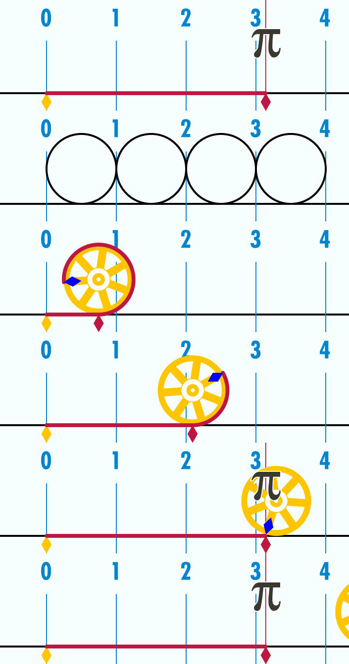
Being irrational means having an infinite decimal representation with no repetition. So, for millennia, mathematicians have tried to improve their understanding of the number π and to obtain its value with greater accuracy.

In this article, we will go through the history of the number π and learn a bit of Python programming along the way.

Definition

#

In the introduction we gave a verbal definition of π and showed an animation that helps visualize it. Now, let’s move on to a mathematical definition. There are several ways to define π mathematically. Here, we will adopt a definition based on calculus.

The circumference of a circle is the length of the arc along its perimeter. Considering, for example, the unit circle given in Cartesian coordinates, we can obtain π as the result of an integral:

Here at Ciência Programada we have a tag just for articles that use SymPy. Let’s see how this Python package handles this integral:

# setup for better outputs in the article, can be ignored
from sympy import init_printing
init_printing(scale=1.05, order='grlex',
              forecolor='Black', backcolor='White', fontsize=10)

from sympy import integrate, Symbol, sqrt, Integral

x = Symbol('x')
expr = 1 / sqrt(1 - x**2)

Integral(expr, (x, -1, 1))

\(\displaystyle \int\limits_{-1}^{1} \frac{1}{\sqrt{- x^{2} + 1}} dx\)

Above, we have the representation of the integral. To solve it, we can use the doit method of the Integral object or call the integrate function directly:

Integral(expr, (x, -1, 1)).doit()

\(\displaystyle \pi\)

integrate(expr, (x, -1, 1))

\(\displaystyle \pi\)

Note that the result of the integral is indeed π.

Now, calculus as we know it today only began to be developed in the 17th century. Before that, how was π defined? Which approximations were used?

Approximations of π

#

Throughout history, many approximations of the value of π have been used. A list in chronological order of approximations of π can be found at this link.

Ancient history

#

The simplest approximation of all is to take the value of π as 3. The Babylonian mathematicians adopted this approximation when appropriate (they knew it was an approximation). And let he who has never used this approximation cast the first stone, engineer :-)

In ancient history, many approximations were used by Babylonians, Egyptians, Greeks, Indians… just to list a few: 25/8, 256/81, 339/108. All of these fractions approximate π with errors smaller than 1 %.

Around 250 BC, the Greek mathematician Archimedes, using the method of exhaustion, showed that the value of π had to be greater than 223/71 and less than 22/7. In this method, polygons are inscribed in and circumscribed about circles, successively increasing the number of sides in order to come ever closer to the shape of the circle.

The figure shows Archimedes’ polygons:

For more details on Archimedes’ work, I recommend the book Arquimedes: uma porta para a ciência (in Portuguese) by Jeanne Bendick, from the incredible Coleção Imortais da Ciência (in Portuguese). Click the links for more details.

About a century later, Ptolemy used the value 377/120, the first known approximation with 3 correct decimal places.

Over the centuries, Archimedes’ geometric method was improved and, by the 17th century, such improvements had already brought the value of π to dozens of correct decimal places.

But what changed in the 17th century? Infinite series.

The revolution of infinite series

#

We already have an article about infinite series on Ciência Programada. Here we will use a bit of what was covered there, so be sure to read it afterwards ;-)

An infinite series is the sum of the terms of an infinite sequence. With equations based on infinite series, a great advance was made in obtaining more precise values for π. Many equations were obtained by many mathematicians, both Eastern and Western. Some equations can be seen here. In this article, we will select just two to illustrate the power of infinite series.

The chosen series are presented below. They were chosen for this article for their didactic value. They are relatively simple expressions by very relevant mathematicians, Gottfried Leibniz and Leonhard Euler. In the links for each mathematician, I included articles that tell a bit about the history of each series, for those who are interested; they are worth reading.

At the beginning of the article, I showed how a symbolic mathematics package like SymPy can be used to represent these summations. My goal now is different: to show how these formulas approach the value of π the more terms are used. I will use very basic Python here, with the standard math library and Matplotlib for plots.

Both series can easily be written as functions, as the next cell shows. Note that the bodies of both functions are similar. A variable, result, is initialized to zero and incremented in loops that depend on the desired number of terms. The return value is the final value of that variable after the loop and the mathematical operations shown in the series expressions.

import math


def pi_leibniz(number_of_terms):
    result = 0
    for k in range(number_of_terms):
        result += 1/((4 * k + 1) * (4 * k + 3))
    return 8 * result


def pi_euler(number_of_terms):
    result = 0
    for k in range(1, number_of_terms + 1):
        result += 1/k**2
    return math.sqrt(6 * result)

With these functions, we can show graphically that the series tend to the value of π as the number of terms used in the summations increases:

import matplotlib.pyplot as plt
from mpl_toolkits.axes_grid1.inset_locator import zoomed_inset_axes
from mpl_toolkits.axes_grid1.inset_locator import mark_inset

plt.style.use('ggplot')
n = range(1, 101)

fig, ax = plt.subplots(figsize=(10, 6))
axins = zoomed_inset_axes(ax, 3, loc='center')

for axis in (ax, axins):
    axis.hlines(math.pi, xmin=min(n), xmax=max(n),
                label='Value of pi',
                linestyle='--', color='red')
    axis.plot(n, [pi_leibniz(i) for i in n],
              label='Leibniz',
              color='green')
    axis.plot(n, [pi_euler(i) for i in n],
              label='Euler',
              color='blue')

x1, y1 = 80, 3.12
x2, y2 = 100, 3.15
axins.set_xlim(x1, x2)
axins.set_ylim(y1, y2)
axins.set_facecolor('whitesmoke')
mark_inset(ax, axins, loc1=2, loc2=4, fc="none", ec="0.6")

ax.legend()
ax.set_ylabel('Approximate value')
ax.set_xlabel('Number of terms')

ax.set_title('Approximation of $\pi$ by series')

plt.show()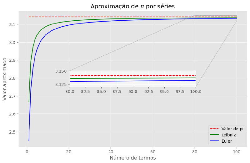

Look at the zoomed-in region of the plot: the two series get closer and closer to the reference value.

It would be interesting to know the percentage error of each approximation. We can create a function to compute the error of a value given a reference value and build a plot of how the error of each series varies:

def error(calculated, expected):
    return (calculated - expected) / expected


from matplotlib.ticker import PercentFormatter, MultipleLocator

fig, ax = plt.subplots(figsize=(10, 6))

ax.plot(n[9:], [error(pi_leibniz(i), math.pi) for i in n[9:]],
        label='Leibniz', color='green')
ax.plot(n[9:], [error(pi_euler(i), math.pi) for i in n[9:]],
        label='Euler', color='blue')

ax.legend()
ax.set_ylabel('Error / %')
ax.set_xlabel('Number of terms')
ax.yaxis.set_major_formatter(PercentFormatter(1, symbol=None))
ax.xaxis.set_major_locator(MultipleLocator(10))

ax.set_title('Approximation of $\pi$ by series - Percentage error')

plt.show()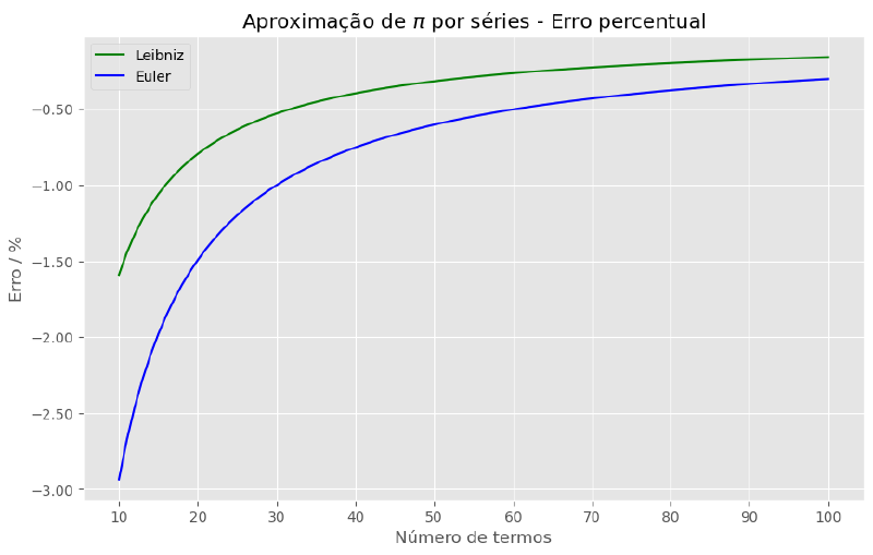

Note how the Leibniz series quickly gives approximations with less than 1 % error. Euler’s needs 30 terms to get into that error range.

In theory, we could keep adding terms to get an ever smaller error:

terms = (100, 500, 1000, 5000)

print('Percentage error x terms')
print('Terms    Leibniz    Euler')

for number in terms:
    error_leibniz = error(pi_leibniz(number), math.pi) * 100
    error_euler = error(pi_euler(number), math.pi) * 100
    print(f'{number:4}   {error_leibniz:.1E}  {error_euler:.1E}')

Percentage error x terms
Terms    Leibniz    Euler
 100   -1.6E-01  -3.0E-01
 500   -3.2E-02  -6.1E-02
1000   -1.6E-02  -3.0E-02
5000   -3.2E-03  -6.1E-03

But what is the limit? How far should we approximate? And, by the way, why get more and more decimal places of π at all?

Why know more decimal places of π?

#

In an article about our atmosphere, I wrote about the importance of not rounding the mathematical constants involved in our calculations. Or, at least, of avoiding drastic rounding, using fewer significant figures than those in our experimental data. This is a bad practice that is propagated in science courses, even at universities. There are well-established standards for rounding and for propagation of uncertainties. Use them.

But what about a value like π, which is irrational? How far is it worth going in obtaining more and more decimal places?

In the following video, mathematician James Grime explains that 39 decimal places of π are enough to calculate the circumference of the observable universe to the precision of a hydrogen atom.

In a recent NASA article, one of the engineers at the agency’s Jet Propulsion Laboratory explains that 15 decimal places are used at the institution. Click the link for details, but basically the engineer explains that this is enough for the precision needed in interplanetary navigation.

As I write this article, the record for the number of decimal places of π is on the order of trillions! And there are motives for the continued search for more digits:

• it is a way to test supercomputers
• to evaluate mathematical algorithms
• to test random number algorithms

And, perhaps, the main motive behind the search is the inherent human desire to break records :-)

How are values with so many decimal places obtained?

Fast-converging series

#

The great technological advances and progress in mathematical studies now give us faster ways to get values of π with the desired precision. The series presented earlier had the problem of needing many terms to reach acceptable error margins. So, there is a cost in processing and memory.

In the early 20th century, the Indian mathematician Srinivasa Ramanujan developed a rapidly converging formula. That formula was a reference for the Chudnovsky brothers, who, a few decades later, developed another series that produces 14 digits of π per term. Here are the formulas:

The mathematics behind each formula goes a bit beyond the scope of this article, but those interested can click the links above. Ramanujan’s formula made it possible to reach records of millions of digits in the 1980s, and the current records of trillions of digits used Chudnovsky’s formula.

We can create Python functions to reproduce these formulas, as in the next cell. Notice that the functions are built very similarly to those for the Leibniz and Euler series:

def pi_ramanujan(number_of_terms):
    result = 0
    for k in range(number_of_terms):
        result += (math.factorial(4 * k) * (1103 + 26390 * k)) / (math.factorial(k)**4 * 396**(4*k))
    return 1 / ((2 * math.sqrt(2) / 9801) * result)


def pi_chudnovsky(number_of_terms):
    result = 0
    for k in range(number_of_terms):
        result += (math.factorial(6 * k) * (13591409 + 545140134 * k)) / (math.factorial(3*k) * math.factorial(k)**3 * (-640320)**(3*k))
    return 1 / ((12 / 640320**(3/2)) * result)

Now, we can redo the comparison plot between the series, adding the two new ones:

fig, ax = plt.subplots(figsize=(10, 6))
axins = zoomed_inset_axes(ax, 3, loc='center')

for axis in (ax, axins):
    axis.hlines(math.pi, xmin=min(n), xmax=max(n),
                label='Value of pi',
                linestyle='--', color='red')
    axis.plot(n, [pi_leibniz(i) for i in n],
              label='Leibniz',
              color='green')
    axis.plot(n, [pi_euler(i) for i in n],
              label='Euler',
              color='blue')
    axis.plot(n, [pi_ramanujan(i) for i in n],
              label='Ramanujan',
              color='orange')
    axis.plot(n, [pi_chudnovsky(i) for i in n],
              label='Chudnovsky',
              color='purple')

x1, y1 = 80, 3.12
x2, y2 = 100, 3.15
axins.set_xlim(x1, x2)
axins.set_ylim(y1, y2)
axins.set_facecolor('whitesmoke')
mark_inset(ax, axins, loc1=2, loc2=4, fc="none", ec="0.6")

ax.legend()
ax.set_ylabel('Approximate value')
ax.set_xlabel('Number of terms')

ax.set_title('Approximation of $\pi$ by series')
plt.show()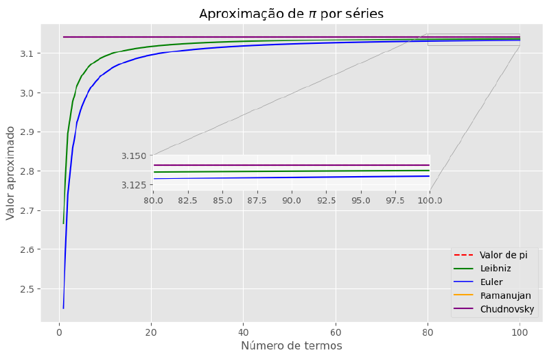

Note that the two new series cannot even be told apart at the scale of the plot, even in the zoomed region. And correct digits are there from the very beginning of both series, overlapping the reference line.

And how do we know the digits are correct?

#

Digit extraction methods have been developed that can be used to check which digit sits at a given position. I plan to write about these methods in the future, but here is the link for those interested.

Reading recommendations

#

For more details on Archimedes’ work, I recommend the book Arquimedes: uma porta para a ciência (in Portuguese) by Jeanne Bendick, from the incredible Coleção Imortais da Ciência (in Portuguese).

For mathematics in general, there is O livro da matemática, the Portuguese edition of DK’s The Maths Book, from the series As grandes ideias de todos os tempos (Big Ideas Simply Explained).

Finally, a good book for Python beginners is Automatize tarefas maçantes com Python (in Portuguese), the Portuguese edition of Automate the Boring Stuff with Python. A book with practical, easy-to-read examples.

Conclusion

#

In this article we saw how to create Python functions to compute summations. More than that, we saw it in the historical context of the study of one of the most famous numbers in mathematics, π. Using Python, we can clearly see how today’s algorithms are more efficient than those developed a few centuries ago. And also how this evolution can be better understood graphically.

See you next time.