Infinite Series - Calculus with Python and SymPy

A good part of the study of calculus is devoted to what are called infinite series. But what, exactly, are infinite series? And how are they related to the paradox of Achilles and the tortoise, one of the so-called paradoxes of Zeno of Elea, the Greek philosopher? What is the connection with quantum mechanics and the uncertainty principle? And where does Python come in? That is what we will find out in this article.

Achilles and the tortoise

#

Achilles, a Greek hero, and a tortoise run a race. Since Achilles is faster than the tortoise, the tortoise is given a head start, beginning the race some distance ahead of Achilles’ starting line. Achilles never overtakes the tortoise, because when he reaches the tortoise’s initial position A, it is already farther ahead, at another position B. When Achilles reaches B, the tortoise is no longer there, because it has advanced to a new position C, and so on, ad infinitum.

The illustration below shows the successive positions:

This is one of the so-called paradoxes of Zeno of Elea (c. 495 - c. 430 BC), a Greek philosopher. Clearly, we know that Achilles will pass the tortoise, as a simple matter of everyday experience. But can you find the flaws in the text above? And, especially, can you formulate the problem mathematically?

Zeno was an Eleatic. The Eleatic school of philosophy rejected the validity of sensory and material experience, holding that only logic should be the criterion for truth. The Eleatics relied on the concept of universal unity and held that sensory experiences are not consistent with that unity, being inconsistent and, at times, contradictory. Only thought could overcome false sensory appearances and reach knowledge of being, the fundamental truth that “all is one”. Moreover, there can be no creation, because being cannot come from non-being, since one thing cannot arise from something that is different from it.

Faced with this, the natural reaction is this:

Uh-huh, quite a hallucinogenic curious way of thinking. I will not go on with this trip into the details of the school, I leave that to the philosophers. However, the last sentence leads to the idea that change is merely an illusion of the senses, and motion is likewise an illusion, a false appearance of mutability, contrary to universal oneness. Hence the origin of the paradox for Zeno. Let us move on to a more mathematical view.

Infinite series, the concept of limit, and the solution of the paradox

#

At its core, the paradox hides the idea of infinity, wouldn’t you agree? As described earlier in its statement, we could keep expanding to other positions: D, E, F… indefinitely. The idea of infinity is not at all trivial and we have already covered it briefly in other articles, to see how it was represented in Python packages such as SymPy.

Another idea that, for many centuries, was considered nontrivial and paradoxical is that an infinite sum can produce a finite result. This idea became easier to understand in the 19th century with the concept of limit and the work of Augustin-Louis Cauchy. Let us look at one of his studies:

In the first line, we express the idea of an infinite sum with the summation symbol. In the second, we take this sum and put a limit with \(n\) tending to infinity, also expressing that limit above the summation symbol. And, for the condition \(0<x<1\), it is possible to obtain an expression for the limit. In other words, the limit, which is for an infinite sum, converges to a finite value when this condition is met. Hence the study of convergence of series, so common in calculus courses. We will return to this subject later in the article.

But what does this have to do with our paradox?

To begin with, let us set some boundary conditions for our problem:

• Achilles starts at an initial position \(x_A\)
• The tortoise starts at an initial position \(x_T\)
• Achilles has a constant speed \(v_A\)
• The tortoise has a constant speed \(v_T\)

Now, the variation of the position, \(x\), of both with time, \(t\), can be expressed by the equations of uniform motion studied in physics:

where \(x_0\) is the initial position of each one and \(v\) is the constant speed of each one.

What are we looking for? Well, we know that, for Achilles to overtake the tortoise, at some position the two will be side by side. How long will this take?

If we have the position equations of both, we can set them equal and solve for the time variable. We just need to solve a simple equation, which we have already seen in previous articles with SymPy. Let us start by importing what we need, creating our symbols, and finding the equality that represents the meeting position of both:

# setup for better outputs in the article, can be ignored
from sympy import init_printing
init_printing(scale=1.05, order='grlex',
              forecolor='Black', backcolor='White', fontsize=10)

from sympy import S, symbols, Eq, solve

xA, xT, vA, vT, t = symbols('x_A x_T v_A v_T t')

meeting_position = Eq(xA + vA * t, xT + vT * t)
meeting_position

\(\displaystyle t v_{A} + x_{A} = t v_{T} + x_{T}\)

With the solve function, we can obtain the expression for the time at which such a meeting will occur:

meeting_time = solve(meeting_position, t)[0]
meeting_time

\(\displaystyle \frac{- x_{A} + x_{T}}{v_{A} - v_{T}}\)

Let us now put in some values to make the subject more tangible. Let us consider that:

• the tortoise was given a head start of 100 m
• Achilles’ speed is 10 m/s
• the tortoise’s speed is 1/10 m/s

The values could be different, I chose these only because they are easier to work out in your head. Substituting into the time expression we obtained, we see that, with a minimum of manipulation, we get an expression compatible with the formula obtained for the limit shown earlier:

That is, the time can be expressed by the following infinite series:

Substituting the values into the SymPy expression, we get the same value:

meeting_time.subs({xA: 0, xT: 100, vA: 10, vT: S('1/10')})  # seconds

\(\displaystyle \frac{1000}{99}\)

With the n method, we can get a numerical approximation of the time needed, in seconds, for our example:

meeting_time.subs({xA: 0, xT: 100, vA: 10, vT: S('1/10')}).n()  # seconds

\(\displaystyle 10.1010101010101\)

If we have an answer, where is Zeno’s error? Well, there are several approaches, but in our calculations what stands out most is that Zeno did not consider time. Since the speeds are different, the time Achilles takes on each stretch is different from the time the tortoise takes, so that eventually he catches up with, and overtakes, the tortoise. Just note in the series that each term is a smaller increment of time. Remember: we are talking about millennia ago, and concepts such as speed were not yet formally defined. The error in Zeno’s statement is the word “never”, which implies time, whereas the entire statement is formulated in terms of distance traveled. There is also the constant change of frame of reference: Achilles -> tortoise -> Achilles… which gives the impression of a fresh start at each point. When we fix the reference, as when we defined the equations of uniform motion, this impression disappears.

Another important thing to notice is that neither the notion of an infinite series nor that of a limit is needed to resolve the paradox. The simple equations of uniform motion are enough. However, formulating the reasoning via time increments leads to important considerations that use concepts that took centuries to be well defined and established.

Let us explore the idea of infinite series in SymPy further.

Representing infinite series in SymPy

#

Let us try to rebuild the summation seen in the paradox example. SymPy has the Sum class, which lets us create a summation:

from sympy import Symbol, oo, Sum, summation

# whenever possible, state the constraints of your symbols
# here, I will consider the constraints of our previous example
a = Symbol('a', positive=True)
n = Symbol('n', positive=True)
x = Symbol('x', positive=True)

expr = a * x**n

s = Sum(expr, (n, 0, oo))
s

\(\displaystyle \sum_{n=0}^{\infty} a x^{n}\)

See how easily we created our summation! However, more than creating it, it would be interesting to be able to obtain symbolic results for it. For that, we have the doit method (literally, “do it!”)

s.doit()

If you want to skip the step of creating the summation and order it done directly, there is the summation function, which does everything in a single step:

s = summation(expr, (n, 0, oo))
s

How interesting. The answer considers two situations, one with \(x<1\) and another where there is no such condition. When \(x<1\) (and greater than zero, an assumption omitted because it was set when the symbol was created with positive=True), we get exactly the expression expected from what we saw in the previous section. For other values of \(x\) there is no convergence, so SymPy simply leaves the expression indicated.

Let us, then, substitute the example values used in the previous section:

s.subs({a: 10, x: S('1/100')})

\(\displaystyle \frac{1000}{99}\)

As expected, the same value as our previous calculations. We can ask for a numerical approximation:

s.subs({a: S('10'), x: S('1/100')}).n()

\(\displaystyle 10.1010101010101\)

This is the power of a symbolic library. See how, by different paths, we got the same result with few commands. Commands that abstract very elaborate concepts, such as that of an equation or of an infinite series.

Understanding the practical importance of infinite series

#

The story of the paradox served to introduce the idea of infinite series in a friendlier way. But what are their real applications?

One of the articles that gave me the most trouble I most enjoyed writing was the one about integrals. In that article, I show that it is important to be aware that much of what calculators, spreadsheets, and the math functions of programming languages present to you are the result of numerical approximations. For example:

from sympy import exp

exp(5)

\(\displaystyle e^{5}\)

See that SymPy left the exponential indicated. We can ask for a numerical value:

exp(5).n()  # equivalent to exp(5).evalf()

\(\displaystyle 148.413159102577\)

How does SymPy obtain such a value? We used the exponential function as an example, but the same question applies to trigonometric functions or, more generally, to transcendental functions.

From a computational point of view, everything tends to be reduced to simpler operations, such as additions and multiplications, since they are fast and have been optimized by software and hardware for many decades. There are several algorithms to approximate functions, such as CORDIC, algorithms based on Chebyshev polynomials, and ones based on Taylor series, just to name a few examples. In practice, a combination of several algorithms may be used depending on the input of the function and its domain. Also, which implementation is used may change depending on the hardware, as discussed in this StackOverflow link.

We see, therefore, that this is a very extensive subject. In this article, we will first talk about the Taylor series. This series is studied in introductory calculus courses because of its simplicity, and several math libraries have implementations of it, as is the case of SymPy.

Taylor series

#

Consider a function that can be expressed by the series

where \(a\) is a constant, as are the coefficients \(c_i\). Assume that the function has continuous derivatives of all orders. Let us evaluate the function and its derivatives at \(x=a\):

Substituting the coefficients into our original function:

which is the so-called Taylor series.

In the specific case where \(a = 0\), we have:

which, in some books, is called the Maclaurin series.

Now, let us recreate all of this in SymPy, that is what you have been reading this for. SymPy has a series function that builds a Taylor series of a function around a given value. It takes a mathematical function, the variable, and the value. Let us create a function with SymPy and the necessary symbols:

from sympy import Function, series

f = Function('f')
a, n, x = symbols('a n x')
series(f(x), x, a)

Exactly what we expected from what we saw throughout the text, just with a different notation. Note that the last term is presented with a Bachmann-Landau notation, indicating that the remaining terms are of order 6 onward. It is possible to remove this notation with the removeO method:

series(f(x), x, a).removeO()

By passing a number as the fourth parameter, we can define the maximum order of the series. For example, passing 3 as the parameter:

series(f(x), x, a, 3)

Since our function has only one variable, \(x\), we can omit it. If we omit the value around which the series expansion is made, it is understood to be zero. Thus:

series(f(x))

We have the Maclaurin series for our function.

We can obtain each term of the series individually as part of a tuple with the args attribute:

series(f(x)).args

SymPy functions have the taylor_term method, to which we pass the order of the desired term and the variable, and we get the expression of that term:

f(x).taylor_term(2, x)

\(\displaystyle \frac{x^{2} \left. \frac{d^{2}}{d \xi^{2}} f{\left(\xi \right)} \right|_{\substack{ \xi=0 }}}{2}\)

Another way to interact with each term of a series is through the lseries method. This method returns a generator, as we see below. If you do not know what a generator is, see this article about generators.

gen_f_taylor = f(x).lseries()
gen_f_taylor

<generator object Expr.series.<locals>.<genexpr> at 0x74d96a121120>

With Python’s next function we can check each term:

next(gen_f_taylor)

\(\displaystyle f{\left(0 \right)}\)

next(gen_f_taylor)

\(\displaystyle x \left. \frac{d}{d \xi} f{\left(\xi \right)} \right|_{\substack{ \xi=0 }}\)

next(gen_f_taylor)

\(\displaystyle \frac{x^{2} \left. \frac{d^{2}}{d \xi^{2}} f{\left(\xi \right)} \right|_{\substack{ \xi=0 }}}{2}\)

Working with generators has several advantages. We can use the islice function from the itertools library, present in standard Python installations. We have already written about islice. Basically, we have control over the next outputs of the generator, without needing to keep using the next function over and over. Let us import the function and check its return, passing our generator and asking for the next 5 outputs of the generator:

from itertools import islice

islice(gen_f_taylor, 5)

<itertools.islice at 0x74d96a1c7f10>

Note that the object generated by islice is also a generator. We can ask for the generator to be fully consumed by passing it to some data structure, for example, a tuple with the tuple function:

tuple(islice(gen_f_taylor, 5))

Let us understand the return we got. We had already started consuming the generator gen_f_taylor, having obtained the first 3 terms of the series. When we passed the value 5 as a parameter to islice, we got the next 5 terms. Since it is an infinite series, we can do this procedure indefinitely, obtaining as many terms as we wish.

To start from the beginning of the series, we can redefine our variable or pass the function directly with the lseries method:

tuple(islice(f(x).lseries(), 5))

Thus, above, we have the first 5 terms of the series.

If we pass 2 numbers to islice, we get the terms from the position of the first number up to the position of the second number. For example, from the third to the seventh term:

tuple(islice(f(x).lseries(), 3, 7))

Thus, we have total control over how we consume our series. Again, if you have not worked with generators before, see the articles mentioned. I tried to be very didactic in them, starting from very simple examples.

Finally, we could get the same generator behavior from the series function simply by passing n=None as one of the arguments:

series(f(x), n=None)

<generator object Expr.series.<locals>.<genexpr> at 0x74d96a32f790>

tuple(islice(series(f(x), n=None), 3))

OK, lots of letters and numbers, let us look at some more practical examples.

Exponential function

#

Let us return to the exponential function example. Let us ask for a Taylor series expansion around \(x = 0\):

series(exp(x))

\(\displaystyle 1 + x + \frac{x^{2}}{2} + \frac{x^{3}}{6} + \frac{x^{4}}{24} + \frac{x^{5}}{120} + O\left(x^{6}\right)\)

Note that, by default, the expansion goes up to the term of order 5, making it explicit that the remaining terms are of order 6 onward. We can change this highest-order term. In the next cell, we pass the function, the variable, the value of \(x\) around which the expansion is made, and the highest-order term:

series(exp(x), x, 0, 8)

\(\displaystyle 1 + x + \frac{x^{2}}{2} + \frac{x^{3}}{6} + \frac{x^{4}}{24} + \frac{x^{5}}{120} + \frac{x^{6}}{720} + \frac{x^{7}}{5040} + O\left(x^{8}\right)\)

And, as already seen, we can remove the order indication of the remaining terms of the series:

series(exp(x), x, 0, 8).removeO()

\(\displaystyle \frac{x^{7}}{5040} + \frac{x^{6}}{720} + \frac{x^{5}}{120} + \frac{x^{4}}{24} + \frac{x^{3}}{6} + \frac{x^{2}}{2} + x + 1\)

Remember, a series is nothing more than an infinite summation. Looking at the result above, we can recognize the general expression of the summation and reproduce it with SymPy:

from sympy import factorial

n = Symbol('n', integer=True)    # important to make clear that it must be an integer
exp_expr = x**n / factorial(n)   # check that this is really the expression
sum_exp = Sum(exp_expr, (n, 0, oo))
sum_exp

\(\displaystyle \sum_{n=0}^{\infty} \frac{x^{n}}{n!}\)

Do you agree with the result?

Now, we can ask SymPy to carry out the summation:

sum_exp.doit()

\(\displaystyle e^{x}\)

Note that SymPy recognizes that the result of this summation is the exponential function. Remember, all of this could have been done in one line of code with summation:

summation(exp_expr, [n, 0, oo])

\(\displaystyle e^{x}\)

Returning to the exp(5) example used earlier, let us see what we get when we ask for the substitution of \(x\) by 5:

summation(exp_expr.subs({x: 5}), [n, 0, oo])

\(\displaystyle e^{5}\)

Thus, if we ask for a numerical approximation coming from the summation, it should equal the one obtained directly from the exp expression:

summation(exp_expr.subs({x: 5}), [n, 0, oo]).evalf(), exp(5).evalf()

\(\displaystyle \left( 148.413159102577, \ 148.413159102577\right)\)

And it really is! Consistent. But what about substitutions from the Taylor series?

We know that the approximation will be better the more terms there are in the series. Let us see this, using the previous value as a reference:

print('n           Taylor          Difference from exp(5)')
print('-'*45)

for i in range(0, 31, 5):
    approx = series(exp(x), x, 0, i).removeO().subs({x: 5}).n()
    approx = float(approx)
    ref = float(exp(5).n())
    print(f'{i:2} {approx:20} {approx-ref:15.4E}')

n           Taylor          Difference from exp(5)
---------------------------------------------
 0                  0.0     -1.4841E+02
 5               65.375     -8.3038E+01
10    143.6894565696649     -4.7237E+00
15   148.37958007973663     -3.3579E-02
20   148.41310786833833     -5.1234E-05
25   148.41315907883663     -2.3740E-08
30   148.41315910257242     -4.1780E-12

See how the difference really does decrease. However, is dozens of terms reasonable for an acceptable difference?

Here we have a disadvantage of the Taylor series approach. Note that we are working with series built around \(x=0\). In the plot below, we see that even lower orders give a good approximation around that value. However, as we move away, as in the case of \(x=5\), the approximation only becomes acceptable with more terms. And, in case you have not noticed yet, for the exponential function it makes no sense to expand around \(x=5\), because the derivative of an exponential is the exponential itself. Around zero this problem does not exist. That is why Maclaurin series are the ones that appear most in exercises, since they avoid problems of this kind. We will come back to discussions along these lines later.

from sympy.plotting import plot
import matplotlib.pyplot as plt
from mpl_toolkits.axes_grid1.inset_locator import zoomed_inset_axes 
from mpl_toolkits.axes_grid1.inset_locator import mark_inset

def move_sympy_plot_to_axes(sympy_plot, plt_ax):
    """Moves a SymPy plot to a Matplotlib axes

    Adapted from: https://stackoverflow.com/a/46813804/8706250

    Parameters
    ----------
    sympy_plot : SymPy plot
    plt_ax : Matplotlib axes
    """

    backend = sympy_plot.backend(sympy_plot)
    backend.ax = plt_ax
    backend._process_series(backend.parent._series, plt_ax, backend.parent)
    backend.ax.spines['right'].set_color('none')
    backend.ax.spines['bottom'].set_position('zero')
    backend.ax.spines['top'].set_color('none')
    plt.close(backend.fig)


fig, ax = plt.subplots(figsize=(10, 6))
axins = zoomed_inset_axes(ax, 128, loc='upper center') # zoom = 128

p_exp = plot(exp(x), (x, -1, 6), show=False, label=r'\\(f(x) = exp(x)\\)')
move_sympy_plot_to_axes(p_exp, ax)
data_exp = p_exp[0].get_points()
# axins.plot(*data_exp)

points = []
points.append(data_exp)

for i in range(0, 31, 5):
    taylor = series(exp(x), x, 0, i).removeO()
    p_taylor = plot(taylor, (x, -1, 6), show=False, label=f"Taylor - order {i}")
    move_sympy_plot_to_axes(p_taylor, ax)
    data_taylor = p_taylor[0].get_points()
    points.append(data_taylor)
    # axins.plot(*data_taylor)

for p in points:
    axins.plot(*p)

x1, y1 = 4.99, 148.0
x2, y2 = 5.005, 148.5
axins.set_xlim(x1, x2)
axins.set_ylim(y1, y2)
mark_inset(ax, axins, loc1=2, loc2=4, fc="none", ec="0.6")

ax.scatter(5, exp(5).n(), color='red', label='Point (5, exp(5))')
axins.scatter(5, exp(5).n(), color='red')

ax.legend()
ax.set_ylim(0, 150)
ax.legend(loc='upper left', bbox_to_anchor=(1, 1))

plt.show()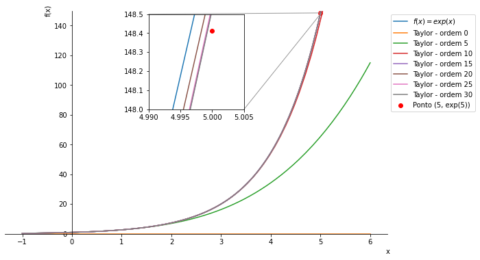

Convergence of series

#

We saw earlier that for a long time the idea that infinite sums can yield finite values was considered paradoxical. And we have already given many examples showing that it is possible to obtain values for some infinite series. Mathematically, such series are convergent. Hence the study of convergence of series and the many convergence criteria and tests seen in calculus courses and books. It is not our place here to go through such tests but, is SymPy able to tell us whether a given sum converges?

Let us create a summation from an expression:

expr = (-1)**(x-1) / x
convergent01 = Sum(expr, (x, 1, oo))
convergent01

\(\displaystyle \sum_{x=1}^{\infty} \frac{\left(-1\right)^{x - 1}}{x}\)

SymPy has an is_convergent method that returns a boolean:

convergent01.is_convergent()

\(\displaystyle \text{True}\)

That is, in this example we have a case that converges. But to what value? Simple, just use the doit method to find out:

convergent01.doit()

\(\displaystyle \log{\left(2 \right)}\)

Let us look at a case of divergence:

expr = 1/(2 * x)
divergent01 = Sum(expr, (x, 1, oo))
divergent01

\(\displaystyle \sum_{x=1}^{\infty} \frac{1}{2 x}\)

divergent01.is_convergent()

\(\displaystyle \text{False}\)

divergent01.doit()

\(\displaystyle \infty\)

Note that the is_convergent method returned False, so that, when we asked for the sum to be carried out, the return was infinity and not a specific value. Consistent with a divergent series.

Usually, in the study of convergent series, the so-called geometric series appear, with the following definition:

from sympy import symbols

u, a = symbols('u a')

geom_series_expr = u**n * a

geom_series = Sum(geom_series_expr, (n, 0, oo))
geom_series

\(\displaystyle \sum_{n=0}^{\infty} a u^{n}\)

Let us see the result of the doit method:

geom_series.doit()

Note that there are two possibilities, which depend on the value of u. Let us make substitutions to illustrate the two possibilities.

# u < 1, should converge:
geom_series.subs({a: 1, u: 1/2}).is_convergent()

\(\displaystyle \text{True}\)

geom_series.subs({a: 1, u: 1/2}).doit()

\(\displaystyle 2\)

Thus, since \(u < 1\), the series converges. In this case, to the value 2.

Looking at a case of divergence:

# u > 1, should diverge
geom_series.subs({a: 1, u: 3/2}).is_convergent()

\(\displaystyle \text{False}\)

geom_series.subs({a: 1, u: 3/2}).doit()

\(\displaystyle \infty\)

The series diverges, hence the indication of infinity in the result.

Parity of functions. Pendulums

#

The parity of functions is a concept linked to symmetry. Even or odd functions can greatly simplify some mathematical manipulations, since patterns appear in terms of series. For more details, see this article about parity of functions. Here, we will see how to recognize whether a function is even or odd from its Taylor series. We will take the opportunity to discuss a few more aspects of these series.

Let us check the Taylor series of the sine function around \(\theta=0\):

from sympy import sin, cos, diff

theta = Symbol('theta')

series(sin(theta))

\(\displaystyle \theta - \frac{\theta^{3}}{6} + \frac{\theta^{5}}{120} + O\left(\theta^{6}\right)\)

The sine and cosine functions can be related through their derivatives. We have already written about derivatives in SymPy:

diff(sin(theta), theta, 1), diff(cos(theta), theta, 1)  # first derivative of each function

\(\displaystyle \left( \cos{\left(\theta \right)}, \ - \sin{\left(\theta \right)}\right)\)

Therefore, in the Taylor series of both functions there must be an alternation of sine and cosine. Let us check:

print('                Sine function')
print('n   d^n(f(x))/dx   d^n(f(x))/dx|x=0   Term')
print('-'*45)

for i in range(8):
    print(f'{i} {diff(sin(theta), theta, i)!s:^15} {diff(sin(theta), theta, i).subs(theta, 0)!s:^15} {sin(theta).taylor_term(i, theta)!s:^15}')

                Sine function
n   d^n(f(x))/dx   d^n(f(x))/dx|x=0   Term
---------------------------------------------
0   sin(theta)           0               0       
1   cos(theta)           1             theta     
2   -sin(theta)          0               0       
3   -cos(theta)         -1          -theta**3/6  
4   sin(theta)           0               0       
5   cos(theta)           1         theta**5/120  
6   -sin(theta)          0               0       
7   -cos(theta)         -1        -theta**7/5040 

We see that in the series, expanded around zero, only terms with odd exponents appear. This is a characteristic of odd functions. One of the many properties of such functions is that \(f(-x) = -f(x)\).

Let us look at the cosine function:

series(cos(theta))

\(\displaystyle 1 - \frac{\theta^{2}}{2} + \frac{\theta^{4}}{24} + O\left(\theta^{6}\right)\)

print('                Cosine function')
print('n   d^n(f(x))/dx   d^n(f(x))/dx|x=0   Term')
print('-'*45)

for i in range(8):
    print(f'{i} {diff(cos(theta), theta, i)!s:^15} {diff(cos(theta), theta, i).subs(theta, 0)!s:^15} {cos(theta).taylor_term(i, theta)!s:^15}')

                Cosine function
n   d^n(f(x))/dx   d^n(f(x))/dx|x=0   Term
---------------------------------------------
0   cos(theta)           1               1       
1   -sin(theta)          0               0       
2   -cos(theta)         -1          -theta**2/2  
3   sin(theta)           0               0       
4   cos(theta)           1          theta**4/24  
5   -sin(theta)          0               0       
6   -cos(theta)         -1         -theta**6/720 
7   sin(theta)           0               0       

We see that in the series only terms with even exponents appear. This is a characteristic of even functions. One of the many properties of such functions is that \(f(-x) = f(x)\).

Let us also show graphically how more terms in the Taylor series widen the range of the domain in which the approximation is acceptable:

from sympy import pi
from matplotlib.ticker import FuncFormatter, MultipleLocator

fig, ax = plt.subplots(figsize=(10, 6))

p_sin = plot(sin(theta), (theta, -2*pi, 2*pi), show=False, label=r'\\(f(\theta) = sin(\theta)\\)')
move_sympy_plot_to_axes(p_sin, ax)

for i in range(0, 13, 2):
    taylor = series(sin(theta), theta, 0, i).removeO()
    p_taylor = plot(taylor, (theta, -2*pi, 2*pi), show=False, label=f"Taylor - order {i}")
    move_sympy_plot_to_axes(p_taylor, ax)

ax.tick_params(axis='both', which='major')



def format_func(value, tick_number):
    """find number of multiples of pi/2"""
    
    N = int(round(2 * value / pi.n()))
    if N == 0:
        return "0"
    elif N == 1:
        return r"\\(\dfrac{1}{2}\pi\\)"
    elif N == 2:
        return r"\\(\pi\\)"
    elif N % 2 > 0:
        return r"\\(\dfrac{{{0}}}{{2}}\pi\\)".format(N)
    else:
        return r"\\({0}\pi\\)".format(N // 2)


ax.xaxis.set_major_locator(plt.MultipleLocator(float(pi.n()) / 2))
ax.xaxis.set_minor_locator(plt.MultipleLocator(float(pi.n()) / 4))
ax.xaxis.set_major_formatter(plt.FuncFormatter(format_func))

ax.set_xlabel(r'\\(\theta\\)')
ax.set_ylabel(r'\\(\sin(\theta)\\)')

ax.set_ylim(-3, 3)
ax.legend()
ax.legend(loc='upper left', bbox_to_anchor=(1, 1))

plt.show()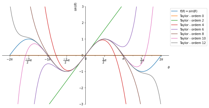

The series was built around \(\theta=0\). Thus, even with few terms we have an acceptable approximation near this value. However, the farther from this value, the larger the error with few terms. Even with more than 10 terms we still do not have an acceptable approximation at the extremes of the domain shown in the figure. It is very important to be aware of this fact.

If you are still having trouble connecting the subject to something more practical, let us look at a common example from physics classes.

You probably studied pendulums in your high school physics classes:

But, in high school, you probably did not see the full equation that represents the motion of the pendulum over time:

After all, the beauty of differential equations is not shown to our young people :-/ Derivation of the equation at this link about pendulums.

In the equation, \(g\) is the gravitational acceleration; \(l\) is the length of the pendulum’s string; and \(\theta\) is the angle of the string with the vertical.

What was probably presented to you is that the variation of the angle and the period are given by:

However, if you later studied differential equations, you will realize that these formulas are not directly obtained from the differential equation. What is often omitted from the student, especially in high school, is that the formulas are only valid for very small angles, usually taken as \(\theta \ll 1\) radian. Now, such an angle is very close to zero and, therefore, we can take few terms of our Taylor series. In fact, we can take just the first term:

If this condition holds, we have

A much simpler equation, from which the formulas presented earlier can be obtained. Do it as an exercise for practice :-)

Notice how the work of solving becomes much simpler with the approximation coming from the Taylor series. Hence the importance of studying it.

Fourier series. Fourier transforms

#

An article about series could not leave out Fourier series and transforms. Fourier transforms are very common in physics and chemistry, consisting of a mathematical manipulation that reorganizes information. You can imagine, for example, that the human eye and ear perform Fourier transforms by analyzing electromagnetic and sound waves, respectively. The subject is quite broad and will certainly appear more times here on the site. Our goal here is to cover the main aspects and see how SymPy performs some basic manipulations. Let us begin with some definitions.

Brief mathematical background

#

General form

#

The most general form of a Fourier series is expressed as a sum of sine and cosine functions:

where the coefficients, which derive from the orthonormal behavior of the sine and cosine functions, are

Fourier series differ from Taylor series in several aspects. Here, two are worth highlighting:

• the interval of convergence is always between \(-\pi\) and \(\pi\) in Fourier series, whereas in Taylor series the interval changes according to the function
• it is rare to find functions that cannot be expanded in a Fourier series, whereas there are more examples of functions that cannot be expanded by Taylor

Changing the interval

#

In some contexts, such as quantum mechanics, it is useful to change the range of a Fourier series from \((-\pi, \pi)\) to \((-L, L)\). For that, the variable \(x\) must be replaced by \(\frac{\pi x}{L}\):

where

DFT

#

We have already seen here on the site that the sine and cosine functions are related to the exponential function through Euler’s formula. And we have also written about complex numbers. So, we can write another form of the Fourier series:

where

In this case, the coefficients are complex and the series will represent only periodic functions. However, it is possible to modify the equation for nonperiodic functions. Consider \(k = \frac{n \pi}{L}\). Now, imagine \(L \to \infty\). As \(L\) increases, changes in \(k\) occur with smaller increments for each change in \(n\). That is, \(\Delta k = \frac{\pi}{L} \Delta n \). In the limit \(\Delta k \to 0\), \(k\) becomes a continuous variable, and the coefficients \(c_k\) can be described as continuous functions of \(k\), \(c(k)\). Therefore, substituting \(\Delta n = \frac{L}{\pi} \Delta k\):

Now, this is the definition of an integral. Setting \(\frac{Lc(k)}{\pi} = \frac{g(k)}{\sqrt{2\pi}}\), we have:

The equation for \(f(x)\) is called the Fourier integral, and \(f(x)\) and \(g(k)\) are called continuous Fourier transforms of each other. For computational calculations, it is sometimes more convenient to work with discrete samples, which gives rise to the discrete Fourier transforms (DFT).

For example, suppose a function of time, such as sine or cosine, expressed as \(\sin(2\pi \nu t)\) or \(\cos(2\pi \nu t)\). Since it is a periodic function, we need samples for only one period \(\tau_0\). The DFT function is defined by

where \(N\) is the number of samples taken from the period \(\tau_0\) and \(k\) ranges from \(-t\) to \(t-1\) in integers centered at zero. The Fourier transform is then said to transform the function from the time domain to the frequency domain. Considering Euler’s formula \(e^{i \theta} = \cos \theta + i \sin \theta\):

Obviously, more samples lead to better outputs. Nowadays there is the fast Fourier transform algorithm, which requires the number of points to be a power of two.

It is convenient to separate the real part from the imaginary part in the previous equation:

The absolute value of \(F(\nu)\) is given by

A plot of \(|F(\nu)|^2\) versus \(\nu\) is called the power spectrum of the Fourier transform.

Difference between Fourier series and Fourier transform

#

Note in the previous subsection that the idea of the Fourier transform arose when a way to obtain series for nonperiodic functions was sought. That is the key point of the distinction.

A Fourier series is used to represent a periodic function through a discrete sum of complex exponentials. A Fourier transform is used to represent a general, nonperiodic function through a continuous superposition or integral of complex exponentials. A Fourier transform can be seen as the limit of the Fourier series of a function as the period approaches infinity, so that the limits of integration change from one period to \((-\infty, \infty)\).

Parity of functions

#

Finally, we saw with Taylor that even or odd functions are convenient because they facilitate some mathematical manipulations. The same occurs in Fourier series.

For odd functions, the coefficients \(a\) are zero and the series becomes

where

For even functions, the coefficients \(b\) are zero and the series becomes

where

That was a very brief review of the subject. It will certainly appear more times here on the site, so many applications will be seen. Now, let us see how SymPy performs Fourier operations.

Fourier series in SymPy

#

We can create a Fourier series for a function with fourier_series:

from sympy import fourier_series

fourier = fourier_series(f(x))
fourier

Note that it was given in the general form, making it clear that it is a sequence of sums.

We can obtain each of the coefficients of the general form:

fourier.a0

\(\displaystyle \frac{\int\limits_{- \pi}^{\pi} f{\left(x \right)} dx}{2 \pi}\)

fourier.an

fourier.bn

We saw in the mathematical background of the previous section that it is common to denote the limit of the interval by \(L\). We can, then, check the limit of the interval:

fourier.L

\(\displaystyle \pi\)

Also in the previous section, we saw that we can write it in exponential form. To do this, we use the rewrite method, requesting that the exp function be used:

fourier.rewrite(exp)

Let us look at some more practical examples.

Plots and function parity

#

Let us take a very simple function as an example: \(f(x) = x\). First, let us create the Fourier series for this function:

from sympy import pi

s = fourier_series(x, (x, -pi, pi))
s

\(\displaystyle 2 \sin{\left(x \right)} - \sin{\left(2 x \right)} + \frac{2 \sin{\left(3 x \right)}}{3} + \ldots\)

As for parity, this function is odd, since \(f(-x) = - f(x)\). From what we saw earlier, the coefficients a should be zero:

s.a0, s.an, s.bn

\(\displaystyle \left( 0, \ \left[0, 0, 0, 0, \ldots\right], \ \left[2 \sin{\left(x \right)}, - \sin{\left(2 x \right)}, \frac{2 \sin{\left(3 x \right)}}{3}, - \frac{\sin{\left(4 x \right)}}{2}, \ldots\right]\right)\)

With the truncate method we can define how many terms we want in our series. For example, with five terms:

s.truncate(5)

\(\displaystyle 2 \sin{\left(x \right)} - \sin{\left(2 x \right)} + \frac{2 \sin{\left(3 x \right)}}{3} - \frac{\sin{\left(4 x \right)}}{2} + \frac{2 \sin{\left(5 x \right)}}{5}\)

The truncate, as used above, shows only nonzero terms. If we pass None to the method, it returns a generator:

gen_fourier = s.truncate(None)
gen_fourier

<generator object SeriesBase.__iter__ at 0x74d969cd09e0>

We can work with this generator using islice, as we did earlier with Taylor series. For example, we can generate the first 10 terms and store them in a tuple:

tuple(islice(gen_fourier, 10))

Note that the first term is zero, referring to the \(a_0\) of the general form of a Fourier series.

And what is the effect of the number of terms? In the plot below, we see that the more terms, the better the approximation of our function:

fig, ax = plt.subplots(figsize=(10, 10))
axins = zoomed_inset_axes(ax, 2, loc='lower right') # zoom = 2

p_x = plot(x, (x, -3, 3), show=False, label=r'\\(f(x) = x\\)')
move_sympy_plot_to_axes(p_x, ax)
data_x = p_x[0].get_points()
axins.plot(*data_x)

for n in range(1, 16, 2):
    fourier = s.truncate(n)
    p_fourier = plot(fourier, (x, -3, 3), show=False, label=f"Fourier - n = {n}")
    move_sympy_plot_to_axes(p_fourier, ax)
    data_fourier = p_fourier[0].get_points()
    axins.plot(*data_fourier)

x1, y1 = -0.5, -0.5
x2, y2 = 0.5, 0.5
axins.set_xlim(x1, x2)
axins.set_ylim(y1, y2)
mark_inset(ax, axins, loc1=1, loc2=2, fc="none", ec="0.6")

ax.legend()
plt.show()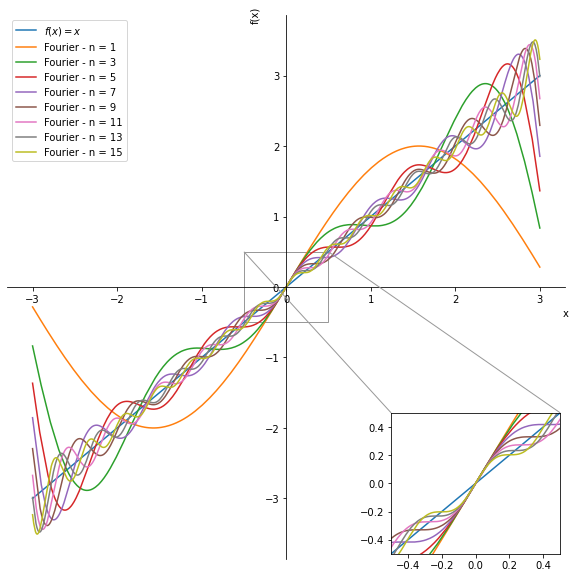

In case it is still not clear, see the following animation:

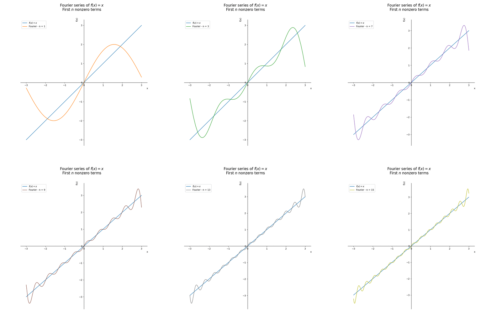
The animation code is in this repository:

chicolucio/fourier

Fourier series demonstration

Python

0

0

Application in electrical engineering

#

To make the practical importance of the subject more evident, let us look at a real application.

A rectifier is an electrical device that converts alternating current into direct current. It has several applications, for example, in power supplies for electronic devices. Let us look at an example of a full-wave rectifier. In this type of rectifier, the input wave is converted into a wave of constant polarity (positive or negative). Mathematically, this corresponds to the absolute value of the function.

Let us create our symbols and the expression for the input wave function:

from sympy import Abs
amplitude = Symbol('A', positive=True, real=True)
period = Symbol('P', positive=True, real=True)
x = Symbol('x', real=True)

expr_input = amplitude * sin((2 * pi / period) * x)
expr_input

\(\displaystyle A \sin{\left(\frac{2 \pi x}{P} \right)}\)

Let us look at the plot of this wave. As an example, let us consider amplitude and period with value 1:

from sympy.plotting import plot

plot(expr_input.subs({period: 1, amplitude: 1}), (x, -2, 2));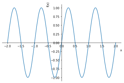

See what an alternating wave looks like. As written earlier, the rectification process is mathematically equivalent to the absolute value of the function. So, let us obtain the expression using SymPy’s Abs function:

expr_output = Abs(expr_input)
expr_output

\(\displaystyle A \left|{\sin{\left(\frac{2 \pi x}{P} \right)}}\right|\)

We can plot this new function, with the same period and amplitude values (which refer to the input function):

plot(expr_output.subs({period: 1, amplitude: 1}), (x, -2, 2));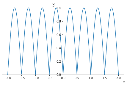

Note that in the plot of the rectified wave there is only the positive part and the period was halved (it went from 1 to 0.5). Thus, the output frequency is twice the input frequency. In case you did not understand, see the figure with both functions overlaid:

p_input = plot(expr_input.subs({period: 1, amplitude: 1}), (x, -2, 2), show=False, label='Input')
p_output = plot(expr_output.subs({period: 1, amplitude: 1}), (x, -2, 2), show=False, label='Output')

fig, ax = plt.subplots(figsize=(12, 6))

move_sympy_plot_to_axes(p_input, ax)
move_sympy_plot_to_axes(p_output, ax)

ax.lines[0].set(linestyle=':', linewidth=3)

ax.legend()
plt.show()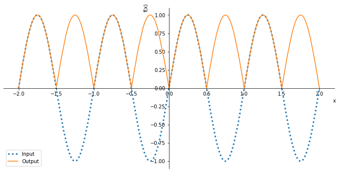

Now, let us obtain our Fourier series (frequency domain) for the rectified wave function (time domain):

s = fourier_series(expr_output, (x, 0, period))
s

\(\displaystyle - \frac{4 A \cos{\left(\frac{4 \pi x}{P} \right)}}{3 \pi} - \frac{4 A \cos{\left(\frac{8 \pi x}{P} \right)}}{15 \pi} + \frac{2 A}{\pi} + \ldots\)

Let us explore the coefficients:

s.a0

\(\displaystyle \frac{2 A}{\pi}\)

s.an

\(\displaystyle \left[0, - \frac{4 A \cos{\left(\frac{4 \pi x}{P} \right)}}{3 \pi}, 0, - \frac{4 A \cos{\left(\frac{8 \pi x}{P} \right)}}{15 \pi}, \ldots\right]\)

s.bn

\(\displaystyle \left[0, 0, 0, 0, \ldots\right]\)

Note how the coefficients \(b_n\) are zero. As we saw earlier, this is characteristic of even functions. The plot confirms that it is an even function, since it is symmetric with respect to the y axis.

Let us substitute values into the function. Just as an example, let us consider amplitude and period with value 1, as done before:

s.subs({period: 1, amplitude: 1}).an

\(\displaystyle \left[0, - \frac{4 \cos{\left(4 \pi x \right)}}{3 \pi}, 0, - \frac{4 \cos{\left(8 \pi x \right)}}{15 \pi}, \ldots\right]\)

See how there is an alternation with zero terms.

Now, let us look at the plot of this series. Since it is a series, we need to define how many terms we will add. Let us start with a low value, such as 5:

plot(s.truncate(5).subs({period: 1, amplitude: 1}), (x, -2, 2));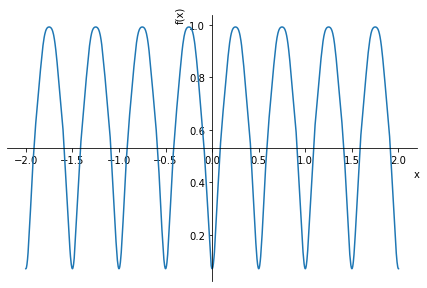

How strange. Our series does resemble the function, but there is a negative part in the plot. Let us plot with more terms. For example, with 10 terms:

plot(s.truncate(10).subs({period: 1, amplitude: 1}), (x, -2, 2));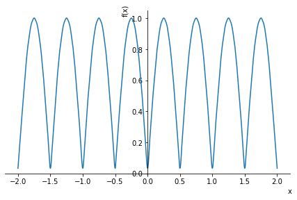

Now we have a better approximation of our function. If you look at the plot, you will see that the minima are not touching the horizontal axis, which would be expected for the given values. If we add more terms, we will have an even better approximation. Let us see with 20 terms:

plot(s.truncate(20).subs({period: 1, amplitude: 1}), (x, -2, 2));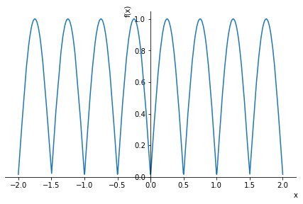

Now the minima are closer to zero. We could keep adding more terms until some approximation criterion was satisfied.

Fourier transforms in SymPy

#

To finish the subject, let us look at the fourier_transform function. Let us start by creating a function:

expr = exp(-x**2)
expr

\(\displaystyle e^{- x^{2}}\)

The function created is a very simple Gaussian. Gaussian functions are widely studied because of their applications in statistics and signal processing. Let us look at its plot:

plot(expr, (x, -5, 5));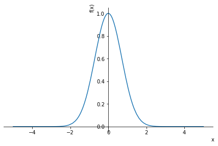

Now, let us do the Fourier transform using the notation shown in the theoretical part of the article:

from sympy import fourier_transform

k = Symbol('k', real=True)
ft = fourier_transform(expr, x, k)
ft

\(\displaystyle \sqrt{\pi} e^{- \pi^{2} k^{2}}\)

See that using the fourier_transform function is very simple. The function we got as output is also a Gaussian. In fact, this is a property of Gaussians. Let us look at the plot of the output function of the transform:

plot(ft, (k, -5, 5));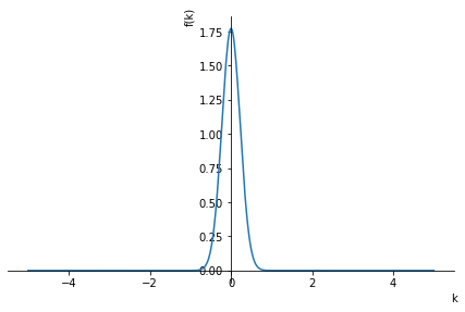

Note that it is a Gaussian with a smaller width than the input Gaussian (before the transform). Let us overlay the plots to make this more evident:

p_input = plot(expr, (x, -5, 5), show=False, label='Input')
p_output = plot(ft, (k, -5, 5), show=False, label='Output')

fig, ax = plt.subplots(figsize=(12, 6))

move_sympy_plot_to_axes(p_input, ax)
move_sympy_plot_to_axes(p_output, ax)

ax.lines[0].set(linestyle=':', linewidth=3)

ax.set_xlabel('')
ax.set_ylabel('')

ax.legend()
plt.show()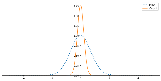

And this is a general property of functions and their Fourier transforms: if a function is more “spread out” in x, its Fourier transform will be more “concentrated” in k. And vice versa. It is not possible to arbitrarily compact both the function and its transform. This is a very informal way of stating an uncertainty principle.

It is quite common to begin the study of Fourier transforms with audio signals, hence the terminology we have already used in this article of saying that the input function is in the time domain and the output one in the frequency domain. Thus, in signal processing, it is said that it is not possible to precisely localize a signal (input function) simultaneously in the time domain and in the frequency domain (output function, Fourier transform).

However, nothing prevents it from being another context. For example, in quantum mechanics the momentum and position wave functions are Fourier transform pairs within a margin of error. Hence the famous Heisenberg uncertainty principle. Not by chance, several Gaussian functions appear during the study of quantum mechanics. In fact, Gaussians are very common in many contexts.

Conclusion

#

Did you imagine it would be possible, in a single text, to go from Greek philosophy to quantum mechanics? And using programming? This article taught me a lot while I wrote it and, I hope, it teaches you a lot too, reader. As important as knowing how to do mathematical operations in a language such as Python is knowing the theoretical background to see the many possible applications. And a bit of history helps, doesn’t it :-)

See you next time.