

The concept of a limit is the most important one in the study of calculus. Many other concepts and ideas are built on the definition of a limit.
In this article, we will see how to find the limit of functions using SymPy and how this package can be a teaching aid in the study of calculus.
Infinity in SymPy #
Before getting into limits themselves, let’s see how the package represents infinity, since limits tending to infinity, or infinity as the answer to a calculus exercise, come up all the time.
As we have seen since the first article of this series on SymPy, it is a symbolic computer algebra system. So we need to know the internal representation of the concept of infinity:
# setup for better outputs in the article, can be ignored
from sympy import init_printing
init_printing(use_latex='png', scale=1.05, order='grlex',
              forecolor='Black', backcolor='White', fontsize=10)

from sympy import oo

type(oo)
sympy.core.numbers.Infinity
Yes, that is two lowercase “o” letters :-)
We can do some simple operations to check whether the results are what we expect based on our mathematical knowledge. Let’s see:
oo + 1\( \infty \)
1000 < ooTrue
1 / oo0
As we see in the last three examples, the results agree with what we expect mathematically. Thus, in a very simple way, we have a representation of a concept that is not trivial.
Now let’s move on to limits.
The limit function
#
The definition of a limit is somewhat abstract, at least at first glance:
The function \(f\) approaches a limit \(l\) near \(a\) means: for every \(\epsilon > 0\) there is some \(\delta > 0\) such that, for all \(x\), if \(0 < |x-a| < \delta\), then \(|f(x) - l| < \epsilon\).
Well… that is quite a tangle of symbols, and it is the starting point of many calculus concepts. But, for this article and for many discussions, we can start from a simpler, more intuitive definition of a limit:
The function \(f\) approaches a limit \(l\) near \(a\) if we can make \(f(x)\) as close as desired to \(l\) by taking \(x\) sufficiently close to, but not equal to, \(a\).
It may still sound abstract, but we will see several examples that should make it easier to understand.
Let’s start with one of the best-known limits, one of the many ways of representing Euler’s number:
$$ e \equiv \lim_{x \to \infty} \left( 1 + \frac{1}{x} \right)^x $$Let’s check whether SymPy returns e for this limit:
from sympy import limit, Symbol

x = Symbol('x')

limit( (1 + 1 / x)**x, x, oo)
e
As we can see, the result is the representation of Euler’s number. To understand it better, let’s look at the following plot:
from sympy.plotting import plot
from sympy import E
import matplotlib.pyplot as plt


def move_sympy_plot_to_axes(sympy_plot, plt_ax):
    """Moves a SymPy plot to a Matplotlib axes

    Adapted from: https://stackoverflow.com/a/46813804/8706250

    Parameters
    ----------
    sympy_plot : SymPy plot
    plt_ax : Matplotlib axes
    """

    backend = sympy_plot.backend(sympy_plot)
    backend.ax = plt_ax
    backend._process_series(backend.parent._series, plt_ax, backend.parent)
    backend.ax.spines['right'].set_color('none')
    backend.ax.spines['bottom'].set_position('zero')
    backend.ax.spines['top'].set_color('none')
    plt.close(backend.fig)


fig, ax = plt.subplots(figsize=(8, 6))

p1 = plot((1 + 1/x)**x, (x, 0, 50), show=False,
          label=r'$\left( 1 + \frac{1}{x} \right)^x$')
p2 = plot(E, (x, 0, 50), show=False, label="Euler's number")

move_sympy_plot_to_axes(p1, ax)
move_sympy_plot_to_axes(p2, ax)

ax.get_lines()[1].set(color='red', linestyle='--')
ax.set_ylim(0, 3)
ax.legend(loc='lower right')

plt.show()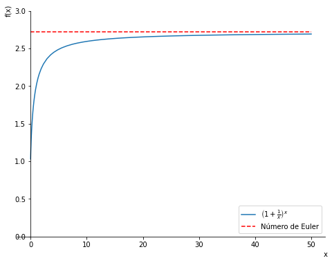
See in the plot how the blue curve approaches the dashed red line, which
represents Euler’s number, as x becomes larger and larger. That is, in the
limit as x tends to infinity, the function approaches the value of Euler’s
number.
One-sided limits #
Let’s look at the plot of the following function f:
$$ f(x) = \frac{1}{x} $$from sympy.plotting import plot
x = Symbol('x')
f = 1 / x
plot(f, (x, -10, 10), ylim=(-10, 10));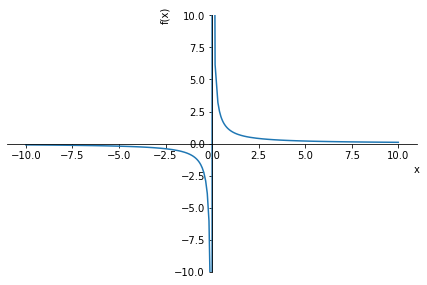
As we can see, the way we approach x=0 affects the limit. This is a case of
one-sided limits. If we approach zero from the right, usually denoted by the
symbol +, we get one limit. Approaching from the left, denoted by the symbol
-, we get another value for the limit. In SymPy, we can indicate the
direction of approach with the dir parameter (for direction) of the limit
function:
limit(f, x, 0, dir='+')\( \infty \)
limit(f, x, 0, dir='-')\( - \infty \)
This parameter only needs to be given in ambiguous cases. For limits tending to infinity (negative and positive), it is not necessary, as we see in the plot:
limit(f, x, -oo), limit(f, x, oo)\( (0, \ 0) \)
Two oscillating functions #
Let’s see a few more examples that usually appear in calculus textbooks. Starting with the function g below:
$$ g(x) = \frac{\sin(x)}{x} $$from sympy import sin, exp
g = sin(x) / x
plot(g, (x, -30, 30));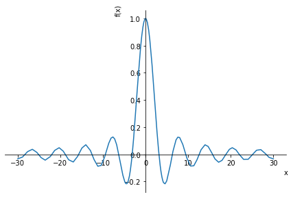
Let’s look at two limits of this function:
limit(g, x, 0)1
limit(g, x, oo)0
That the limit as x tends to zero is 1 is quite evident from the plot. The limit as x tends to infinity becomes more evident when we widen the x axis range a bit, which is why I specified the range from -30 to 30 in the code. See how the function oscillates between positive and negative values, but the amplitude of the oscillation gets smaller and smaller as the values of x become more positive or more negative. Thus, in the limit as x tends to infinity, whether positive or negative, the function approaches zero.
The function h defined below can be analyzed similarly:
$$ h(x) = \frac{\sin(x)^2}{x} $$h = sin(x)**2 / x
plot(h, (x, -30, 30));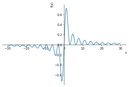
limit(h, x, 0)0
limit(h, x, oo)0
The limit as x tends to zero is evident in the plot. The limit as x tends to infinity can be analyzed like the previous function g. The difference is that the amplitude decreases during the oscillation, tending to zero, but the sign of the function does not change.
Which function dominates? #
Let’s look at the function j defined below:
$$ j(x) = \frac{\exp(x)}{x^{100}} $$Let’s start with the plot:
# only to turn off the numerical error warning
import warnings
warnings.filterwarnings('ignore', category=RuntimeWarning)

j = exp(x) / (x**100)

plot(j);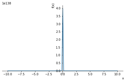
See how the vertical scale of the plot extends to values on the order of \(10^{138}\). This makes it hard to analyze and understand the limit values we want to evaluate. Let’s make some plots with more suitable scales. We start by restricting the ranges of x and y:
plot(j, (x, -2, 2), ylim=(0, 10));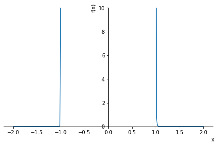
Now we have a slightly better idea of the behavior of the plot. We see that near \(x = \pm 1\) the function grows very quickly. Let’s check the results of the following four limits, comparing them with the plot shown:
limit(j, x, 0)\( \infty \)
limit(j, x, 1)e
limit(j, x, -oo)0
limit(j, x, oo)\( \infty \)
The first three limits are evident from the plot and from the expression of the function, don’t you agree? Near zero, the function tends to infinity; near 1 the function tends to e (substitute 1 into the function if you have trouble seeing it in the plot); and, when x tends to negative infinity, the function tends to zero, consistent with the plot showing the curve close to the x axis. What seems strange is the last limit, when x tends to positive infinity. After all, the plot shows the curve hugging the x axis, which leads us to believe the result should also be zero.
To understand it, let’s start by plotting the numerator and denominator functions:
h_numerator = exp(x)
plot_h_numerator = plot(h_numerator, (x, -2, 2),
                        ylim=(0, 100), show=False, label='Numerator')
h_denominator = x**100
plot_h_denominator = plot(h_denominator, (x, -2, 2),
                          ylim=(0, 100), show=False, label='Denominator')

fig, (ax1, ax2) = plt.subplots(nrows=1, ncols=2, figsize=(8, 6))

move_sympy_plot_to_axes(plot_h_numerator, ax1)
move_sympy_plot_to_axes(plot_h_denominator, ax2)

ax1.set_title('Numerator - $\exp(x)$ \n')
ax2.set_title('Denominator - $x^{100}$ \n')

plt.show()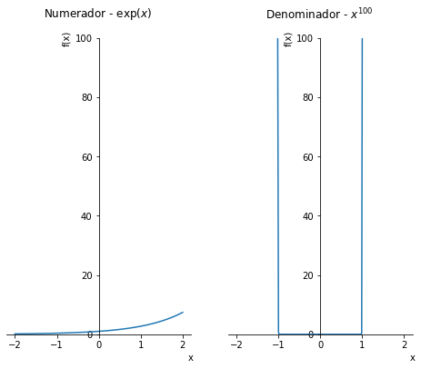
In the range shown, the denominator function grows very quickly near \(x \pm 1\). We also see that the exponential function in the numerator is increasing. Now, if the numerator function is increasing, it may happen that at some point it becomes larger than the denominator. But, before checking this numerically, let’s recall some usual discussions in the study of mathematical functions.
When we evaluate functions that result from sums, differences, products or quotients of other functions of different types, or of different powers of the same type of function, it is usual to say that one function “dominates” the other. This means that when x tends to negative or positive infinity, the plot of the function will resemble that of the dominant function. Thus, we have the following rules of thumb, usually discussed and detailed in calculus courses:
- exponential functions dominate polynomial functions
- polynomial functions dominate logarithmic functions
- among exponential functions, larger bases dominate smaller bases
- among polynomial functions, higher orders dominate lower orders
Therefore, in the case at hand, the exponential function in the numerator will dominate the polynomial function in the denominator. This means it makes sense for the function j to tend to infinity as x tends to infinity, since the exponential function is increasing. But the plot of j, at least in the window shown, does not show this happening; it seems to tend to zero…
Well, at some point the numerator must equal the denominator and then become larger than it. To find the point (or points) where this equality occurs, we just need to solve the following equation:
$$ \exp(x) - x^{100} = 0 $$We can use the solve function already presented in this series of articles:
from sympy import solve

solution = solve(exp(x) - x**100, x, numerical=False)
[s.n() for s in solution]
\( 1.01015271985388, \ -0.990147384359501, \ 647.2775124394 \)
We see that there are three values of x that satisfy the equation. Note that the last one is particularly high, well above the range shown in the previous plots. Let’s make a plot overlaying the numerator and denominator functions over a range of x values surrounding the value found:
fig, ax = plt.subplots(figsize=(8, 6))

h_numerator = exp(x)
plot_h_numerator = plot(h_numerator, (x, 600, 650), show=False)
h_denominator = x**100
plot_h_denominator = plot(h_denominator, (x, 600, 650), show=False)

p1 = plot_h_numerator
p2 = plot_h_denominator

move_sympy_plot_to_axes(p1, ax)
move_sympy_plot_to_axes(p2, ax)

ax.legend(loc='upper left')

plt.show()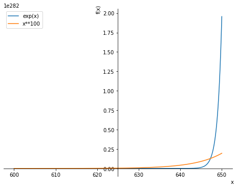
Now we do see that the exponential function really dominates from x of about 647.3 on. Thus, we can redo the plot of the function j with a more suitable scale to visualize this fact:
plot(j, (x, 640, 650), axis_center=(640, 0));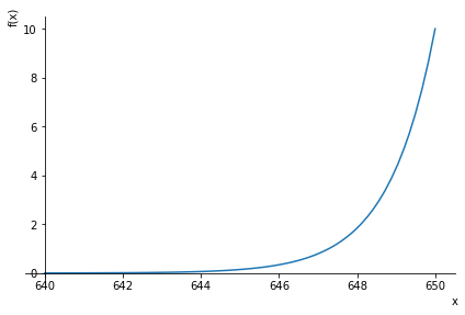
We see that, indeed, the function starts to increase and, in the limit as x tends to infinity, tends to infinity.
We can also check these changes in the behavior of the function by substituting some example values:
examples = (-1000, -2, -1, -0.9, -0.1, 0.1, 0.9, 1,
            1.01, 1.1, 2, 100, 500, 600, 650, 1000)

row_length = 35


print(f'x {" " * (row_length//2)} | {" " * (row_length//2)} j(x)')
print('-' * 45)

for number in examples:
    value = (exp(number) / number**100).n()
    spaces = str(row_length - len(str(number)))
    print(f'{number:<{spaces}}{value:.3e}')
x | j(x)
---------------------------------------------
-1000 5.076e-735
-2 1.068e-31
-1 3.679e-1
-0.9 1.531e+4
-0.1 9.048e+99
0.1 1.105e+100
0.9 9.260e+4
1 2.718e+0
1.01 1.015e+0
1.1 2.180e-4
2 5.829e-30
100 2.688e-157
500 1.779e-53
600 5.775e-18
650 1.000e+1
1000 1.970e+134
Notice how the values really do move away from values near zero to large values as x increases. Interesting, right?
The Squeeze Theorem #
To wrap up this article, we will see the so-called Squeeze Theorem, also known as the Sandwich Theorem. Let’s start with the formal statement:
Let \(I\) be an interval having the point \(a\) as a limit point. And let g, f and h be functions defined on \(I\) except possibly at \(a\). Suppose that for every \(x\) in \(I\) not equal to \(a\) we have
$$g(x) \le f(x) \le h(x)$$and suppose also that
$$ \lim_{x \to a} g(x) = \lim_{x \to a} h(x) = L $$Then
$$\lim_{x \to a} f(x) = L $$
OK, very abstract. Let’s see an example, starting from the following function:
$$ k(x) = x^2 \sin \left( \frac{1}{x} \right) $$Let’s start with the plot of the function:
k = x**2 * sin(1/x)

plot(k, (x, -0.25, 0.25));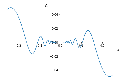
Graphically, we see that the limit of this function as x tends to zero must be zero. Let’s see the result from SymPy:
limit(k, x, 0)0
Expected result. But so what?
If you wanted to solve the exercise by hand, you would probably start with the following limit property:
$$ \lim_{x \to a} (f(x) \cdot g(x)) = \lim_{x \to a} f(x) \cdot \lim_{x \to a} g(x) $$However, \(\lim\limits_{x \to 0} \sin \left( \frac{1}{x} \right)\) does not exist. So another way of solving it must be adopted.
From the very definition of the sine function, we have: \(-1 \le \sin \left( \frac{1}{x} \right) \le 1\). It follows, therefore, that \(-x^2 \le x^2 \sin \left( \frac{1}{x} \right) \le x^2\). Since \(\lim\limits_{x \to 0} -x^2 = \lim\limits_{x \to 0} x^2 = 0\), the squeeze theorem gives \(\lim\limits_{x \to 0} x^2 \sin \left( \frac{1}{x} \right) = 0\).
We can use SymPy to visually check the meaning of what we have just seen:
fig, ax = plt.subplots(figsize=(8, 6))

p1 = plot(k, (x, -0.25, 0.25), show=False,
          label=r'$x^2 \sin \left( \frac{1}{x} \right)$')
p2 = plot(-x**2, (x, -0.25, 0.25), show=False, label='$-x^2$')
p3 = plot(x**2, (x, -0.25, 0.25), show=False, label='$x^2$')

move_sympy_plot_to_axes(p1, ax)
move_sympy_plot_to_axes(p2, ax)
move_sympy_plot_to_axes(p3, ax)

ax.legend(loc='upper left')

plt.show()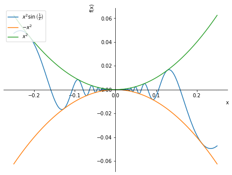
We see how the plot of our function of interest lies between the plots of the other functions. Hence the name “sandwich” :-)
Conclusion #
That was a good calculus review, wasn’t it? We saw several examples that are usual in calculus classes and how using SymPy lets us enrich the discussion further, thanks to how easily it generates plots and obtains results that are not always quickly evident, leading to deeper discussions.
See you next time.


