

Engineers and scientists are always trying to get the most performance out of their equipment and projects at the lowest cost. This search gives rise to so-called optimization problems. In this article, we will see how to use Python, with the help of the SymPy package, to solve them.
Understanding an optimization problem #
Let’s start by understanding the essence of an optimization problem from a mathematical point of view. We can think of optimization as the search for an input to a function \(f(x)\) such that the result is the best output value of \(f(x)\). And what would this “best value” be? Usually, it means the maximum value (if the function represents something positive, such as profit) or the minimum value (if the function represents something undesirable, such as cost).
In the article on derivatives with Python, we saw that the derivative of a function is related to the slope of a line tangent to the function at a given point. Thus, when \(f^{\prime}(x) = 0\), that slope is zero, indicating that we are at a maximum or a minimum. Points that satisfy the previous equality are called critical points of a function.
The second derivative, \(f^{\prime\prime}(x)\), is related to the curvature of \(f(x)\), and we can use it to check whether a given critical point is a maximum or a minimum. If \(f^{\prime\prime}(x) < 0\), the function has a maximum; if \(f^{\prime\prime}(x) > 0\), the function has a minimum; and if \(f^{\prime\prime}(x) = 0\), the function is at an inflection point, changing from a region of maximum to one of minimum, or vice versa.
Let’s go through an example. Consider the following function:
$$ f(x) = x^3 - 2x^2 + x $$Let’s create it with SymPy:
# setup for better outputs in the article, can be ignored
from sympy import init_printing
init_printing(scale=1.05, order='grlex',
              forecolor='Black', backcolor='White', fontsize=10)

# importing what we need for the start of this article
from sympy import Symbol, diff, solve, plot

# creating the variable symbol and the function
x = Symbol('x')
f = x**3 - 2*x**2 +x
f
\(\displaystyle x^{3} - 2 x^{2} + x\)
With SymPy’s diff function, we can easily obtain the first and second
derivatives:
first_derivative = diff(f, x)
first_derivative
\(\displaystyle 3 x^{2} - 4 x + 1\)
second_derivative = diff(f, x, 2)
second_derivative
\(\displaystyle 2 \left(3 x - 2\right)\)
With the solve function, we can obtain the critical points by solving the
first derivative for x. That is, by solving \(f^{\prime}(x)=0\):
critical_points = solve(first_derivative, x)
critical_points
\(\displaystyle \left[ \frac{1}{3}, \ 1\right]\)
Note that the result comes out as a list. We can substitute each result into the expression of the second derivative:
second_derivative.subs({x: critical_points[0]}), second_derivative.subs({x: critical_points[1]})\(\displaystyle \left( -2, \ 2\right)\)
And check whether there is any inflection point:
inflection_point = solve(second_derivative, x)
inflection_point
\(\displaystyle \left[ \frac{2}{3}\right]\)
We see that \(f^{\prime\prime}(\frac{1}{3}) < 0\), indicating a maximum, and that \(f^{\prime\prime}(1) > 0\), a minimum. At \(x = \frac{2}{3}\) the concavity of the function changes.
Let’s look at the graph of the function:
plot(f, (x, -0.2, 1.2));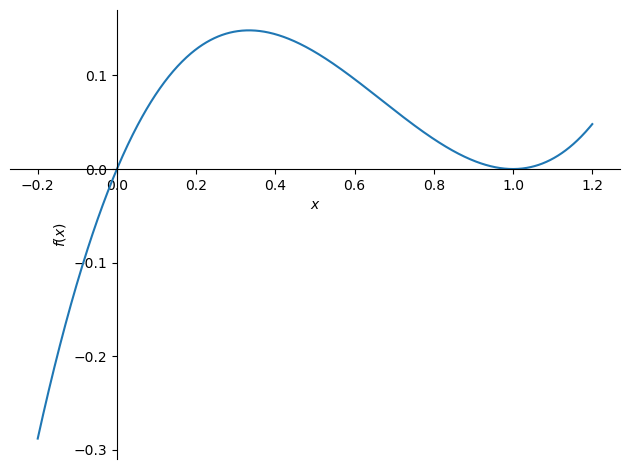
Note that the graph was deliberately built over an interval (domain) in which the maximum and the minimum are evident. However, observe that the function is increasing for \(x > 1\) and decreasing for \(x < 0\). Hence the importance of defining a domain of validity for the problem right at the start. Assuming a domain such that \(x \in [0, 1]\), we can state that \((\frac{1}{3}, f(\frac{1}{3}))\) is a maximum.
Application example: minimizing costs #
Let’s take a very common example in chemical processes: minimizing the cost of building a tank. By the way, I am a chemist by training, and I have already written here a bit about how technology influenced my career, just as it certainly influences yours. For more details on my projects, see my portfolio.
Obtaining our function #
In our example, we will consider a cylindrical tank of fixed volume (V), and we want to determine the length (L) and the diameter (D) that minimize the cost of the tank. The cost per unit area of the side of the tank is \(c_s\), and the cost per unit area of the top and bottom of the tank is \(c_t\). With a bit of basic geometry, shown in the following figure, we can obtain our function \(f\), which represents the cost:
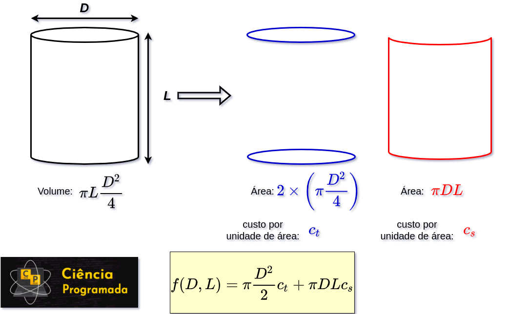
Let’s create the symbols needed to represent our function. Note that all of them were given the restriction of being positive values, since it makes no sense to talk about negative dimensions or costs. It is important to remember to evaluate restrictions in optimization problems.
from sympy import pi

diameter = Symbol('D', positive=True)
length = Symbol('L', positive=True)
volume = Symbol('V', positive=True)
side_cost = Symbol('c_s', positive=True)
top_cost = Symbol('c_t', positive=True)

f = side_cost * pi * diameter * length + top_cost * (pi / 2) * diameter**2
f
\(\displaystyle \frac{\pi D^{2} c_{t}}{2} + \pi D L c_{s}\)
Let’s assume there is no limit on the values and look for an expression in terms of V and D. Thus, eliminating L from the expression:
cylinder_volume = (pi / 4) * diameter**2 * length
cylinder_volume
\(\displaystyle \frac{\pi D^{2} L}{4}\)
length_from_volume = solve(cylinder_volume - volume, length)[0]
length_from_volume
\(\displaystyle \frac{4 V}{\pi D^{2}}\)
f = f.subs({length: length_from_volume})
f
\(\displaystyle \frac{\pi D^{2} c_{t}}{2} + \frac{4 V c_{s}}{D}\)
Therefore, the expression above is the one we want to optimize, obtaining a minimum value. Let’s obtain the expression of its first derivative with respect to the diameter:
f_min = diff(f, diameter)
f_min
\(\displaystyle \pi D c_{t} - \frac{4 V c_{s}}{D^{2}}\)
Now, we can obtain an expression for the diameter that makes the derivative zero:
optimal_diameter = solve(f_min, diameter)[0]
optimal_diameter
\(\displaystyle \frac{2^{\frac{2}{3}} \sqrt[3]{V} \sqrt[3]{c_{s}}}{\sqrt[3]{\pi} \sqrt[3]{c_{t}}}\)
And, with the diameter, obtain the optimal length:
optimal_length = length_from_volume.subs({diameter: optimal_diameter}).simplify()
optimal_length
\(\displaystyle \frac{2^{\frac{2}{3}} \sqrt[3]{V} c_{t}^{\frac{2}{3}}}{\sqrt[3]{\pi} c_{s}^{\frac{2}{3}}}\)
Let’s see which length / diameter ratio minimizes the cost:
optimal_length / optimal_diameter\(\displaystyle \frac{c_{t}}{c_{s}}\)
Note how interesting this result is. If the costs are the same, the cylinder that minimizes the cost is the one whose length equals the diameter of its base, since the ratio above would be 1. We will write more about this below.
Let’s plug in example values to better visualize our result. We will consider the costs equal to 1 unit and the volume equal to 10 units. The diameter that minimizes the function is:
solve(f_min.subs({side_cost: 1, top_cost: 1, volume: 10}), diameter)[0]\(\displaystyle \frac{2 \sqrt[3]{5}}{\sqrt[3]{\pi}}\)
Which, numerically, corresponds to:
# the _ lets us retrieve the value of the previous cell
_.n()
\(\displaystyle 2.33508864988147\)
Let’s look at the graph of our cost function:
p = plot(f.subs({side_cost: 1, top_cost: 1, volume: 10}),
     (diameter, 0, 5), ylim=(0, 100), legend=True, show=False)

p[0].label = 'f'
p.show()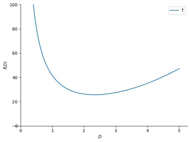
Note how there really is a minimum around a diameter of 2.33. Therefore, this is the diameter (and also the length) for the given boundary conditions.
What if the costs are different? #
What happens if the costs are different? Let’s consider the cost of the side of the tank to be twice the cost of the top:
solve(f_min.subs({side_cost: 2, top_cost: 1, volume: 10}), diameter)[0]\(\displaystyle \frac{2 \sqrt[3]{10}}{\sqrt[3]{\pi}}\)
_.n()\(\displaystyle 2.94202734335627\)
Note that the diameter of the base increased compared to the previous case. Consequently, since the length / diameter ratio depends only on the costs, the length is half the diameter obtained. Can you now understand the “flattened” shape of the cylinders that store liquids, which we usually see in industrial plants?
In these cylinders, the internal pressure of the liquid is given by the famous equation \(P = \rho g h\), that is, it depends on the density of the liquid, on gravity, and on the height of the liquid column. Therefore, a tall tank would require thicker walls to withstand the pressure of the liquid. And, of course, this greatly affects construction costs, especially of the side walls. Simple, right? Of course, there is much more involved, as can be seen here.
And what about all those different shapes of food cans? #
We saw in the calculations above that, if the costs of the side and of the top are equal, the cylindrical shape that minimizes the total cost is the one whose base diameter equals the length of the cylinder. But then why is that shape so rare among the canned goods we see on the market? In fact, first of all, why a cylinder?
In our calculations, we implicitly considered that the cost comes only from the area. So why not use spherical containers? After all, one of the first things taught in geometry classes is that the sphere has the smallest surface area of all closed shapes around a given volume. OK, cool… Now try stacking several spherical containers on a supermarket shelf. Good luck :-)
Besides the fact that spheres roll very easily, their packing is inefficient. At most, we can fill 74% of the available space by stacking spheres. Look for your nearest trusted chemist if you want a mathematical proof of that. Thus, it is clear that other considerations are involved. It is not just the construction cost; there is also the cost of transport, storage, and disposal. In this sense, more cylindrical shapes turn out to be more interesting. Besides the ergonomic factor, your customer needs to be able to hold what they are going to consume. Can you imagine having to hold a soda can with both hands because its diameter is large?
In the can manufacturing process, the greatest waste is at the top and bottom, because of the need for cutting and welding. Of course, there is recycling, but that makes the cost different, and in that case the cost of the side is lower, which makes taller cans make sense.
Conclusion #
Besides calculus and programming, we also had a crash course on packaging ;-)
We saw the care that must be taken in optimization problems, from the correct identification of the domain, through the boundary conditions, to the critical analysis of the results obtained. And the whole process was quite agile thanks to SymPy.
See you next time.


