Mass Balance with Python and SymPy

Mass balance equations are important for practically all calculations in solving chemical engineering problems. For this reason, they will be present throughout your undergraduate course and professional career. Mass balances are carried out during the operation of processing plants over different periods of time, with the goal of controlling processes, maintaining production, and increasing efficiency.

In this article, we will solve two mass balance problems using the SymPy library and review some important principles.

The Concept of Mass Balance

#

Mass balance is the application of the Law of Conservation of Mass:

Therefore, when the process is continuous and operates at steady state, the accumulation inside a piece of equipment is zero:

Remember, a continuous process is one in which mass passes continuously across the system boundaries. A steady-state process, in turn, is one in which the values of the process variables do not change with time.

With a relatively simple equation we can represent, in general form, the balance of any quantity:

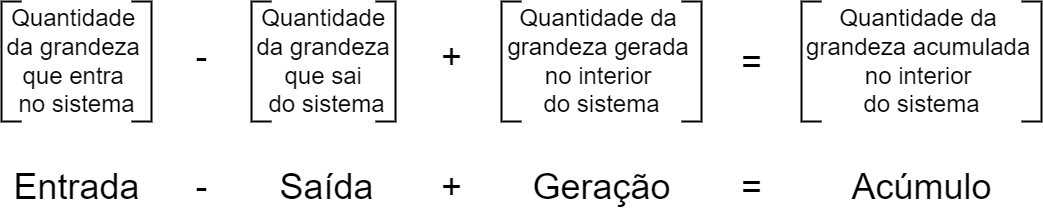
In terms of a balance of a quantity across the system boundaries:

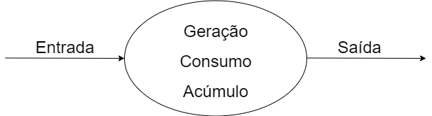
Analyzing a real case

#

Let’s analyze a simple problem. Suppose that 100 mol/h of a mixture with 30% of component A and 70% of component B is separated by distillation into two fractions. The top stream contains 70% of component A and the bottom stream has 20% of component B. Let’s calculate the molar flow rate of each stream.

The first step in solving a molar balance problem is to draw the process diagram, specifying the boundaries and adding the known variables:

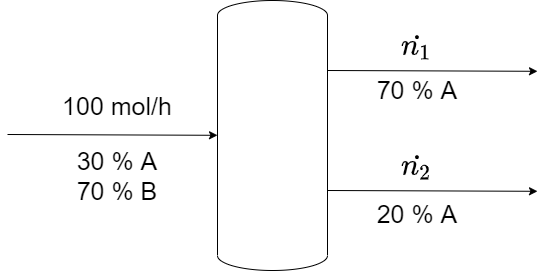
After analyzing the figure, we see that there is crossing of the process boundaries, so this problem operates as a continuous process. Also, the values of the process variables do not change with time, so it is at steady state. Furthermore, we note that no chemical reaction takes place.

Solving with Python and SymPy

#

To solve the problem, let’s import the libraries we will use:

from collections import namedtuple
import sympy
sympy.init_printing(use_latex='png', scale=1.05, order='grlex',
                    forecolor='Black', backcolor='White', fontsize=10)

Let’s start by creating the variables with the information from the problem statement and completing them with the mole fractions that were not given, but that are easily determined from the following constraints:

Where x_a is the mole fraction of component A and x_b that of component B, both in the top stream. y_a is the mole fraction of component A and y_b that of component B, both in the bottom stream.

feed_rate = 100  # molar flow rate in mol/h

Composition = namedtuple('Composition', 'A B')

feed = Composition(0.3, 0.7)      # feed composition
stream_1 = Composition(0.7, 0.3)  # top stream composition
stream_2 = Composition(0.2, 0.8)  # bottom stream composition

Note that I used the namedtuple function. It lets us access values using field names instead of the position indices of a tuple, which makes the code more readable. In case that is not clear yet, we will see it applied right below.

Now, let’s define the molar flow rate symbols using LaTeX. We usually put a dot above the flow symbol to denote a rate. Thus, the molar flow rate (\(\dot{n}\)) of a process stream is the number of moles (\(n\)) transported per unit of time.

flow_rate_1, flow_rate_2 = sympy.symbols('\dot{n_1} \dot{n_2}')

flow_rate_1, flow_rate_2

\( (\dot{n_1}, \ \dot{n_2}) \)

The next step is to write the equations we need to solve in terms of the known variables and the unknowns. Since there is no chemical reaction in this problem and it involves a molar balance at steady state, we have:

This is consistent with what we wrote at the beginning of the article about the accumulation term inside a piece of equipment being zero:

Therefore, for our exercise, the overall molar balance is:

And the component molar balance is:

We need to pass this information to SymPy by creating a system of equations. We have already written about this in this article; let’s apply it to our exercise:

system = (sympy.Eq(flow_rate_1 + flow_rate_2, feed_rate),                                     # overall
          sympy.Eq(stream_1.A * flow_rate_1 + stream_2.A * flow_rate_2, feed.A * feed_rate),  # component A
          sympy.Eq(stream_1.B * flow_rate_1 + stream_2.B * flow_rate_2, feed.B * feed_rate)   # component B
         )  

# showing each equation of the system
for equation in system:
    display(equation)

In Python, the symbols = and == are the assignment and equality operators, respectively, and we cannot use them to create equalities in equations. To set up an equation, SymPy has the Eq function, which creates a symbolic equality.

Another important point is that we can see the advantage of using the namedtuple function when we access the components. We named the fields A and B and accessed the values using dot notation, which improves the readability of the code.

With the system created, we just need to ask for it to be solved with SymPy’s solve function:

solution = sympy.solve(system)
solution

\( \{ \dot{n_1}: 20.0, \ \dot{n_2}: 80.0 \} \)

So, the top stream has a flow rate of 20 mol/h and the bottom stream has a flow rate of 80 mol/h.

This line of reasoning applies to any number of components. As long as the number of independent equations is equal to the number of unknowns, the system can be solved. Let’s look at one more example, this time with 3 outlet streams and 3 components.

A real case with more components

#

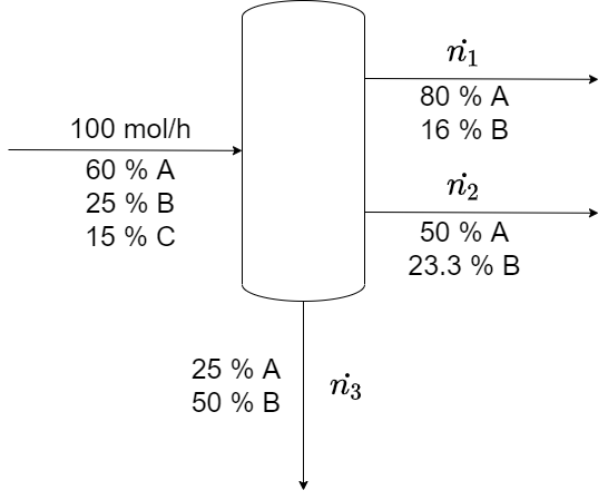
Suppose that 100 mol/h of a mixture with 60% of component A, 25% of component B, and 15% of component C is separated by distillation into three fractions. The streams contain:

i) 80% of component A and 16% of component B;
ii) 50% of component A and 23.3% of component B;
iii) 25% of component A and 50% of component B.

Let’s calculate the molar flow rate of each stream. To do so, we start by drawing the process diagram, specifying the boundaries and adding the known variables:

Solving with Python and SymPy

#

We need to create the variables with the information needed to solve the problem. Let’s extract this data from the problem statement, and the remaining mole fractions can be determined from the following constraints:

feed_rate = 100  # molar flow rate in mol/h

Composition = namedtuple('Composition', 'A B C')

feed = Composition(0.6, 0.25, 0.15)        # feed composition
stream_1 = Composition(0.8, 0.16, 0.04)    # top stream composition
stream_2 = Composition(0.5, 0.233, 0.267)  # middle stream composition
stream_3 = Composition(0.25, 0.5, 0.25)    # bottom stream composition

Now, let’s define the molar flow rate symbols using LaTeX:

flow_rate_1, flow_rate_2, flow_rate_3 = sympy.symbols('\dot{n_1} \dot{n_2} \dot{n_3}')
flow_rate_1, flow_rate_2, flow_rate_3

\( \dot{n_1}, \ \dot{n_2}, \ \dot{n_3} \)

In this problem:

Based on that, let’s write the equations we need to solve. The line of reasoning is the same as in the previous case; only the number of variables and equations grows.

The overall molar balance is:

And the component molar balance is:

Now let’s pass this information to SymPy by creating a system of equations:

system = (sympy.Eq(flow_rate_1 + flow_rate_2 + flow_rate_3, feed_rate),
          sympy.Eq(stream_1.A * flow_rate_1 + stream_2.A * flow_rate_2 + stream_3.A * flow_rate_3, feed.A * feed_rate),
          sympy.Eq(stream_1.B * flow_rate_1 + stream_2.B * flow_rate_2 + stream_3.B * flow_rate_3, feed.B * feed_rate),
          sympy.Eq(stream_1.C * flow_rate_1 + stream_2.C * flow_rate_2 + stream_3.C * flow_rate_3, feed.C * feed_rate))

# showing each equation of the system
for equation in system:
    display(equation)

After creating the system, we need to ask for it to be solved with SymPy’s solve function:

solution = sympy.solve(system)
solution

\( \{ \dot{n_1}: 50.0404203718674, \ \dot{n_2}: 29.9110751818917, \ \dot{n_3}: 20.0485044462409 \} \)

The top stream has a flow rate of 50 mol/h, the middle stream 30 mol/h, and the bottom stream 20 mol/h.

Conclusion

#

Solving mass balance equations got simpler with Python, didn’t it?! In this article, we saw how some features of the SymPy library automate the solution of mass balance problems. Moreover, we can easily apply the tools used here to solve other types of balances and chemical engineering problems.

This article is a collaboration between me, Helena Benevenuto, and Ciência Programada. Follow me on LinkedIn for more chemistry content.

Share this article on your networks and follow the Ciência Programada project to stay up to date. See you next time.