

Imagine you are on vacation in the city of Königsberg, in 18th-century Prussia. The Pregel River divides the city into four distinct regions, connected by seven bridges. The challenge occupying the minds of the locals is seemingly simple: would it be possible to take a walk through the city crossing each of the seven bridges exactly once?
This question, which looks like a trivial pastime, gave rise to one of the most applied fields of modern mathematics: graph theory.
The Königsberg Bridge Problem #
In 1736, the Swiss mathematician Leonhard Euler received this challenge and realized that the geographic question (the exact positions of the bridges, the distances between the islands) was irrelevant. All that mattered was the structure of the connections: which regions were linked by bridges and how many bridges connected them.
The map below shows the actual layout of the seven bridges over the Pregel River, the starting point of Euler’s reasoning.

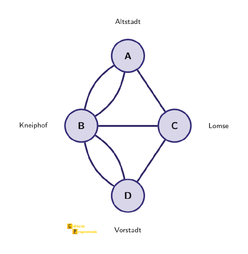
Euler abstracted the problem: he represented each region as a point and each bridge as a line connecting two points. With this representation, the question became: is it possible to traverse every line of this diagram exactly once, in a single continuous route?
Euler’s model
Labeling each region with a letter, we count its bridges:
- A (Altstadt, north bank): 3 bridges
- B (Kneiphof, central island): 5 bridges
- C (Lomse, east island): 3 bridges
- D (Vorstadt, south bank): 3 bridges
Result: all four “points” have an odd number of connections.
Königsberg was the German name of the city; since 1946 it has been called Kaliningrad and belongs to Russia.
- Altstadt (lit. “old town”): north bank of the Pregel River
- Kneiphof: central island of the Pregel, now called Kant Island, where the cathedral in which Immanuel Kant is buried stands
- Lomse: island east of Kneiphof, separated by an arm of the river
- Vorstadt (lit. “suburb”): south bank of the Pregel River
The graph below represents this abstraction, with vertices in place of the regions and edges in place of the bridges. The two parallel edges between A and B (and between B and D) represent the two bridges that existed between those regions.
Euler’s answer was no, and he showed it with a simple argument. Notice that, each time the walker enters a region by one bridge, they must leave by another. Every passage through an intermediate region therefore consumes a pair of bridges. This means that any region that is neither the starting point nor the end point must have an even number of bridges. Only the start and the end of the route can have an odd number. In Königsberg, however, all four points have an odd number of bridges, which would require four start or end points at the same time, something impossible in a single continuous route.
More precisely: a route that traverses each edge exactly once is called an Eulerian trail. If it returns to the starting point, it is an Eulerian circuit, and for one to exist, all vertices must have even degree. If it starts and ends at distinct points, exactly two vertices may have odd degree. In Königsberg, with four vertices of odd degree, neither condition is satisfied. In the article Paths, Cycles, and Connectivity, we will formalize the distinction between walk, trail, and path; in Eulerian and Hamiltonian Graphs, we will see the rigorous proof of this result and its generalizations.
Two of the seven bridges were destroyed in the bombings of World War II, and two others were demolished afterward; of the three that remained, only two date from Euler’s time. Today there are five bridges in the same places as in the original problem. With this configuration, two vertices have degree 2 and the other two have degree 3, and today it is possible to cross all the existing bridges exactly once, starting on one island and ending on the other. The structure changed and the answer changed with it, which illustrates that in graph theory the answer depends on the structure, not on the geography.
This work, published in the paper Solutio problematis ad geometriam situs pertinentis (1736), is considered the birth of graph theory (see the entry Seven Bridges of Königsberg).
What Is a Graph? #
The central idea that Euler developed is very simple:
A graph is a set of vertices (points, nodes) and a set of edges (lines, connections) that link pairs of vertices.
There is no geometry, no coordinates, no distances: only the structure of who is connected to whom.
This abstraction seems like an impoverishment, but it allows the same theory to apply to completely different domains.
Another Example: the Four Color Theorem #
The Bridges of Königsberg are not the only classic problem that the language of graphs clarifies. Consider any geographic map: a political map, a neighborhood map, a board divided into regions. We want to color the regions so that two countries (or neighborhoods) that share a border never have the same color. How many colors are needed?
This question was raised in 1852 by the mathematician Francis Guthrie, while he was coloring a map of the counties of England, and it remained open for 124 years. Intuitively, it seems that four colors should be enough for any planar map, but proving it turned out to be very hard.
The connection with graph theory is immediate: just represent each region as a vertex and draw an edge between two vertices whenever the corresponding regions share a border. The map coloring problem then becomes a graph coloring problem: assign colors to the vertices so that adjacent vertices receive different colors.
The following figure illustrates this abstraction with a map of four regions (A, B, C and D) that are mutually adjacent, each colored with a distinct color, and the corresponding graph, where all the edges reflect the adjacencies of the map.
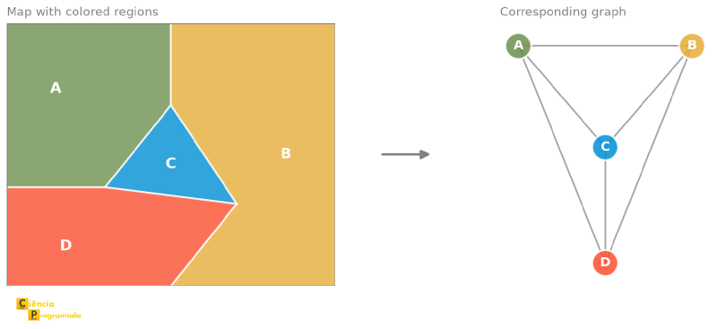
In this specific example, the four regions are all mutually adjacent: A borders B, C, and D; B borders A, C, and D; and so on. The resulting graph is K₄, the complete graph on four vertices, in which every pair of vertices is connected by an edge. To color it, we necessarily need four colors.
Every planar map can be colored with at most four colors so that neighboring regions (those that share a border of positive length) receive distinct colors.
What makes this theorem remarkable is its proof. In 1976, Kenneth Appel and Wolfgang Haken published a proof that reduced the problem to a finite (but enormous) set of cases to check, and used a computer to verify all of them. It was the first major mathematical proof to depend on a computer, and it sparked a philosophical debate about what it means to “prove” something in mathematics that continues to this day (see the entry Four color theorem).
Two geometric facts lie behind the statement:
- In any planar map, it is impossible to have five mutually adjacent regions (which would require the graph K₅, which is not planar).
- The graph K₄ we saw above is planar (it can be drawn in the plane without crossings) and shows that four colors are sometimes necessary.
These two facts, however, do not prove that four colors suffice: a map may need more colors than its largest group of mutually neighboring regions suggests. A small example is a central region surrounded by a ring of five regions. In this map there are no four mutually neighboring regions, and yet four colors are needed: the ring, with an odd number of regions, already uses up three, and the central region, which neighbors all of them, needs a fourth. It is precisely this easy intuition, that everything comes down to how many regions touch at the same time, that no one managed to turn into a proof during the 124 years the problem remained open.
The theory of planar graphs and Kuratowski’s planarity criterion will be discussed in detail in the article Planar Graphs, which also returns to coloring: the Four Color Theorem stated for graphs, a proof that six colors always suffice, and applications in scheduling.
Why Are Graphs So Useful? #
Graph theory is a universal language for modeling relationships between objects. The key is to realize that, in many real problems, what matters is not the objects themselves, but the connections between them.
Computer Science #
- Computer networks: routers are vertices, cables are edges. Finding the shortest path between two routers is a graph problem.
- Operating systems: dependency graphs between processes help detect deadlocks.
- Compilers: a program’s control-flow analysis uses directed graphs.
- Databases: the entity-relationship model is essentially a graph.
- Search algorithms: BFS (breadth-first search) and DFS (depth-first search) are algorithms on graphs.
Engineering and Logistics #
- Electrical networks: identifying circuits, analyzing energy flow.
- Route planning: the Traveling Salesman Problem asks for the Hamiltonian cycle of least cost in a weighted graph.
- Construction projects: precedence graphs determine the order of activities (PERT/CPM method, Program Evaluation and Review Technique / Critical Path Method).
Natural and Social Sciences #
- Chemistry: molecules are graphs where atoms are vertices and chemical bonds are edges. Structural isomers have the same atoms linked in different ways (their graphs are not isomorphic), and recognizing whether two structural formulas describe the same molecule is a graph isomorphism problem.
- Biology: protein-protein interaction networks, food webs (who eats whom), phylogenetic trees.
- Sociology: social networks, where people are vertices and friendships are edges. The concept of “six degrees of separation” is a statement about the diameter of a graph.
- Epidemiology: modeling the spread of diseases in contact networks.
The Internet and Social Networks #
The World Wide Web itself is an enormous graph, but with a difference from the Königsberg graph and the map coloring graph, both undirected: it is a directed graph. Each page is a vertex and each hyperlink is an edge with a direction. If Page A points to Page B, that does not imply that B points to A. Direction matters: the number of pages that point to a vertex (its in-degree) is a direct measure of how referenced (and potentially relevant) that page is.
The following graph illustrates a mini-web with five pages. The arrows indicate the direction of the hyperlinks, and the size of each node is proportional to the PageRank computed by the algorithm, which anticipates a result that is not immediately obvious.
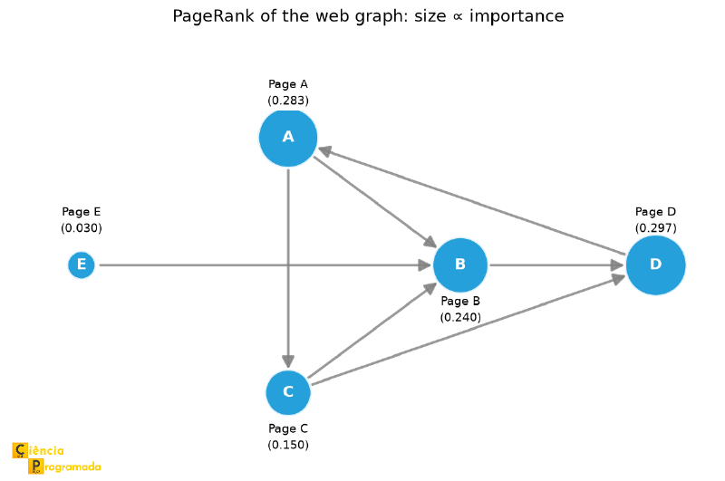
In this example, Page \(B\) receives links from three distinct pages (\(A\), \(C\), and \(E\)), and is the most referenced in terms of in-degree. Page \(E\), on the other hand, receives no incoming links. There is also a cycle: following \(A \to C \to D \to A\), the navigator returns to the starting point. These properties (in-degree, absence of incoming links, and cycles) are exactly what PageRank models, with results that sometimes surprise.
PageRank is the algorithm developed by Larry Page and Sergey Brin at Stanford University in 1996, which became the basis of Google’s search engine. The central idea is the random surfer model: imagine an internet user who, at each step, randomly chooses one of the links on the current page and follows it. The PageRank of a page is the probability that this surfer is on it after a very large number of steps, that is, a measure of how frequently the page is visited in the long run.
$$PR(A) = \frac{1-d}{N} + d \sum_{v \to A} \frac{PR(v)}{L(v)}$$where \(d \approx 0.85\) is the damping factor (the probability of continuing to click instead of “starting over” on a random page), \(N\) is the total number of pages, and \(L(v)\) is the number of links leaving \(v\). Pages that receive many links from pages that are themselves highly ranked accumulate high PageRank, an iterative process that converges to a stable distribution.
The animation below shows this convergence process: the circles represent pages, the size of each circle indicates the PageRank computed in the current iteration, and the arrows represent the hyperlinks.

The name “PageRank” is a double play on words: it honors Larry Page, one of its creators, and it describes what the algorithm does, which is to rank pages (pages). The original 1998 paper, The Anatomy of a Large-Scale Hypertextual Web Search Engine, is a widely cited reference in the field.
Computing the PageRank of our mini-web. To apply the algorithm to the graph in the diagram above, we need to build the transition matrix \(M\), a \(5 \times 5\) matrix where the entry \(M_{ij}\) represents the fraction of the PageRank of page \(j\) that is transferred to page \(i\) at each step. The construction rule is straightforward: if page \(j\) has \(k\) outgoing links and one of them points to \(i\), then \(M_{ij} = \frac{1}{k}\); otherwise, \(M_{ij} = 0\). Since each page distributes all of its weight among its outgoing links, each column of \(M\) sums to 1.
Numbering the nodes as \(A=0\), \(B=1\), \(C=2\), \(D=3\), \(E=4\) and reading the edges of the graph:
- Column \(A\) (\(A\) has 2 outgoing links: to \(B\) and \(C\)): \(M_{BA} = 0.5\), \(M_{CA} = 0.5\), all others = 0.
- Column \(B\) (\(B\) has 1 outgoing link: to \(D\)): \(M_{DB} = 1.0\).
- Column \(C\) (\(C\) has 2 outgoing links: to \(B\) and \(D\)): \(M_{BC} = 0.5\), \(M_{DC} = 0.5\).
- Column \(D\) (\(D\) has 1 outgoing link: to \(A\)): \(M_{AD} = 1.0\).
- Column \(E\) (\(E\) has 1 outgoing link: to \(B\)): \(M_{BE} = 1.0\).
The row of \(E\) is entirely zero: no one points to \(E\), so \(E\) only receives the teleportation “floor” \(\frac{1-d}{N}\).
$$M = \begin{pmatrix} 0.0 & 0.0 & 0.0 & 1.0 & 0.0 \\ 0.5 & 0.0 & 0.5 & 0.0 & 1.0 \\ 0.5 & 0.0 & 0.0 & 0.0 & 0.0 \\ 0.0 & 1.0 & 0.5 & 0.0 & 0.0 \\ 0.0 & 0.0 & 0.0 & 0.0 & 0.0 \end{pmatrix} \quad \text{(rows: } A, B, C, D, E \text{; columns: } A, B, C, D, E\text{)}$$Connection with the previous formula. Recall the PageRank formula presented above:
$$PR(A) = \frac{1-d}{N} + d \sum_{v \to A} \frac{PR(v)}{L(v)}$$The matrix \(M\) was built precisely to represent this summation. The entry \(M_{ij}\) captures the term \(\frac{PR(j)}{L(j)}\): when \(j\) links to \(i\), \(M_{ij} \cdot PR(j) = \frac{PR(j)}{L(j)}\); otherwise it is zero. The product \(M \cdot \mathbf{PR}\) in row \(i\) adds up all these contributions, which is precisely \(\sum_{v \to i} \frac{PR(v)}{L(v)}\). Therefore, the scalar formula above is equivalent to the vector equation
$$\mathbf{PR} = \frac{1-d}{N} \mathbf{1} + d M \mathbf{PR}$$where \(\mathbf{1}\) is the vector of ones and \(\mathbf{PR}\) is the vector of ranks.
The following algorithm solves this equation by the power iteration method:
it starts with the uniform distribution \(\mathbf{w} = \tfrac{1}{N}\mathbf{1}\) and
repeatedly applies \(\mathbf{v} = d M \mathbf{w} + \tfrac{1-d}{N}\mathbf{1}\)
until convergence, which corresponds exactly to the line
v = M_hat @ w + (1 - d) / N in the code below.
With the matrix in hand, we can apply the algorithm to our mini-web. The resulting vector contains the normalized PageRanks (sum = 1) of \(A\), \(B\), \(C\), \(D\), and \(E\), respectively:
import numpy as np

def pagerank(M, d=0.85):
    N = M.shape[1]
    w = np.ones(N) / N        # initial uniform distribution
    M_hat = d * M
    v = M_hat @ w + (1 - d) / N
    while np.linalg.norm(w - v) >= 1e-10:
        w = v
        v = M_hat @ w + (1 - d) / N
    return v

# M[i][j] = fraction of the links of j that point to i
M = np.array([
    [0.0, 0.0, 0.0, 1.0, 0.0],  # A receives 100% from D
    [0.5, 0.0, 0.5, 0.0, 1.0],  # B receives 50% from A, 50% from C, and 100% from E
    [0.5, 0.0, 0.0, 0.0, 0.0],  # C receives 50% from A
    [0.0, 1.0, 0.5, 0.0, 0.0],  # D receives 100% from B and 50% from C
    [0.0, 0.0, 0.0, 0.0, 0.0],  # E receives from no one
])

pages = ["A", "B", "C", "D", "E"]
ranks = pagerank(M)
for page, rank in sorted(zip(pages, ranks), key=lambda x: -x[1]):
    print(f"Page {page}: {rank:.4f}")
Page D: 0.2974
Page A: 0.2828
Page B: 0.2395
Page C: 0.1502
Page E: 0.0300The result is counterintuitive: \(B\) has the highest in-degree (it receives links from \(A\), \(C\), and \(E\)), but it is not the node with the highest PageRank. \(D\) and \(A\) come out ahead. Why? \(B\) passes 100% of its rank to \(D\) (since its only outgoing link points to \(D\)). \(D\), in turn, passes 100% to \(A\). And \(A\) redistributes to \(B\) and \(C\), which feed \(D\) again. The cycle \(D \to A \to C \to D\) and \(D \to A \to B \to D\) creates a feedback loop that accumulates rank in \(D\) and \(A\) over the iterations. \(B\) receives a lot, but also gives away a lot, keeping nothing for itself.
\(E\) confirms the opposite case: with no incoming links, its PageRank is just the teleportation “floor,” \(\frac{1 - 0.85}{5} = 0.03\), regardless of where it points.
Social networks are also modeled as graphs, but with an important distinction regarding the direction of the edges. On Facebook, friendship is mutual by definition: if Alice is a friend of Bob, Bob is a friend of Alice, and the graph is undirected. On Instagram or Twitter/X, following someone does not imply being followed back: the graph is directed, with the edge A→B indicating “A follows B”.
The following graph models a small social network with six users and friendship relations, and is therefore undirected.
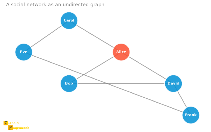
Alice and David have degree 3 (the highest local connectivity in the network) and form, together with Bob, a triangle: the three are mutual friends. Carol is connected only to Alice and Eve; Frank, only to David and Eve. It is already possible to see that some vertices concentrate more connections than others and that the position of a vertex in the network influences its ability to “reach” the others in a few hops. This notion of centrality (how strategically positioned a vertex is in the network) is one of the central metrics in social network analysis.
A famous result in this context is the six degrees of separation hypothesis: the idea that any two people in the world are at most six “hops” apart in the global social network. In 2011, Facebook researchers analyzed the platform’s social graph (then with more than 700 million users) and found an average distance of 4.74 hops between two users (3.74 intermediaries), below the six of the hypothesis, in a real-scale network.
The Beauty of Abstraction #
Graph theory operates at the pure level of structure. A benzene molecule, a social network with ten thousand users, and the São Paulo subway map can all be modeled as graphs and studied with the same mathematical tools.
Euler did not know, in 1736, that he was founding a theory that would be central to computing, telecommunications, bioinformatics, and social network analysis in the following centuries. He just wanted to solve a puzzle about bridges.
In the next article, we will formalize the language of graph theory: definitions, notation, and the first fundamental examples.
The Articles in the Series #
Throughout this series, we will build the foundations of graph theory systematically. We will start with the basic definitions and move on to deep results and their applications:
- Graphs: A Language for Modeling Connections (this article)
- Definitions and Notation in Graph Theory: the formal language (vertices, edges, neighborhood, subgraphs, complete graphs)
- Degree of a Vertex and the Handshaking Lemma: degree, regular graphs, and the theorem that relates degrees and edges
- Isomorphism and Matrix Representation: when two graphs are “the same” and how to represent them computationally
- Paths, Cycles, and Connectivity: how to navigate a graph; bipartite graphs and their characterization
- Trees: connected, acyclic graphs, widely used in computing
- Eulerian and Hamiltonian Graphs: special routes that traverse all edges or all vertices
- Planar Graphs: when a graph can be drawn without edge crossings
- Directed Graphs: when the direction of the connections matters


