

So far, we have dealt with graphs whose relations are symmetric: if \(A\) is connected to \(B\), then \(B\) is also connected to \(A\). But many real-world relations are asymmetric.
A one-way street goes from \(A\) to \(B\), but not from \(B\) to \(A\). A hyperlink leads from one page to another, but the other page does not necessarily point back. A task \(A\) must be completed before \(B\) starts, and not the other way around.
To model these situations, we need directed graphs.
Why Do Digraphs Matter? #
Whenever a relation between two objects is not automatically reciprocal, an ordinary graph is not enough: we also have to record its direction. Some examples:
- Navigation and maps: one-way streets and air routes cannot always be traveled in both directions
- The web and search engines: hyperlinks point from one page to another, and Google’s PageRank (already seen in Graphs: A Language for Modeling Connections) is built on this structure
- Social networks: following someone on Instagram or X does not imply being followed back
- Compilers and package managers: dependencies between modules can only be resolved in a specific order
- Task scheduling: a project with steps that must happen in sequence
To make the idea concrete before the formal definition, consider the following scenario.
Example: a one-way city block
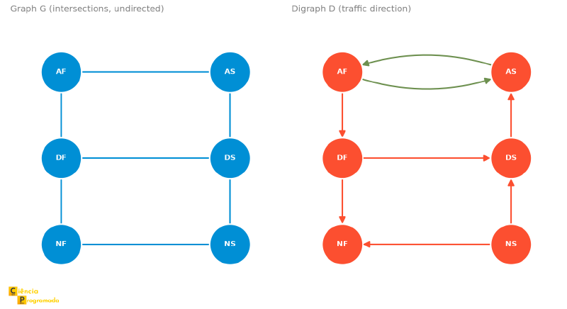
Problem: Consider a block in Copacabana, in Rio de Janeiro, bounded by four streets (Avenida Atlântica, Rua Figueiredo Magalhães, Avenida Nossa Senhora de Copacabana, and Rua Santa Clara) with Rua Domingos Ferreira cutting the block in half. Model this block first as an ordinary graph \(G\) and then as a digraph \(D\), recording the traffic direction of each street.
Solution: Each intersection is a vertex, identified by the two streets that cross there: \(AF\) (Atlântica × Figueiredo), \(AS\) (Atlântica × Santa Clara), \(DF\) (Domingos Ferreira × Figueiredo), \(DS\) (Domingos Ferreira × Santa Clara), \(NF\) (N. S. Copacabana × Figueiredo), and \(NS\) (N. S. Copacabana × Santa Clara). Each stretch of street between two neighboring intersections is an edge.
Ignoring the traffic direction, this is already an ordinary graph \(G\), with edges
$$(AF,AS), (AF,DF), (DF,DS), (DF,NF), (DS,AS), (NS,DS), (NF,NS)$$But the streets have traffic directions: Av. Atlântica is two-way; Rua Figueiredo Magalhães is one-way in the direction \(AF \to DF \to NF\); Rua Santa Clara is one-way in the opposite direction, \(NS \to DS\) and \(DS \to AS\); Rua Domingos Ferreira flows from \(DF\) to \(DS\); and Av. Nossa Senhora de Copacabana flows from \(NS\) to \(NF\). Recording each direction as an arc, we get the digraph
$$D: \{(AF,AS), (AS,AF), (AF,DF), (DF,NF), (NS,DS), (DS,AS), (DF,DS), (NS,NF)\}$$The digraph is the same block, now with the information about where traffic can go on each street. The figure below shows the two versions side by side:
What Is a Digraph? #
A digraph \(D = (V, E)\) is a pair where:
- \(V\) is a finite nonempty set of vertices
- \(E\) is a set of arcs: ordered pairs of distinct vertices
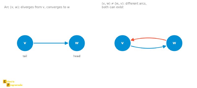
For an arc \((v, w) \in E(D)\):
- \(v\) is the tail (starting point)
- \(w\) is the head (end point)
- We say the arc diverges from \(v\) and converges to \(w\)
- In the geometric representation, we draw an arrow from \(v\) to \(w\)
In a (undirected) graph, the edge \(\{u,v\} = \{v,u\}\), with no distinction.
In a digraph, the arc \((u,v) \neq (v,u)\): they are different arcs! Both can exist at the same time.
Concrete example
Problem: For the digraph \(D\) with \(V = \{a, b, c, d, e\}\) and \(E = \{(a,b),(b,c),(a,e),(b,e),(e,b),(e,c),(d,c),(d,e)\}\), describe the adjacency relations of each vertex.
Solution:
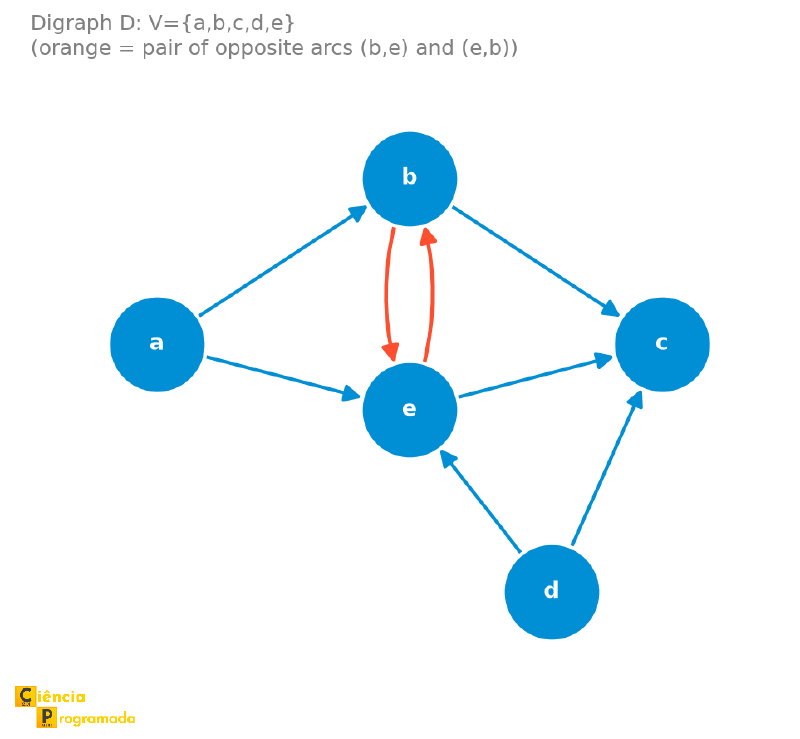
- \(a\): points to \(b\) and \(e\) (but nobody points to \(a\))
- \(b\) and \(e\) have arcs in both directions between them: \((b,e)\) and \((e,b)\)
- \(c\): receives arcs from \(b\), \(e\), and \(d\), but points to nobody
Underlying Graph and Orientation #
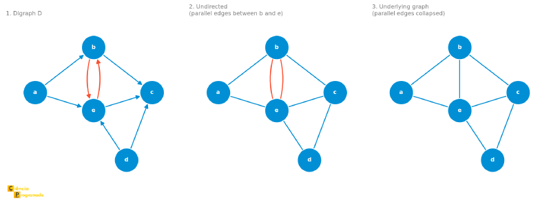
The underlying graph of a digraph \(D\) is obtained by removing the directions of the arcs (turning them into undirected edges) and eliminating the resulting parallel edges.
Example: building the underlying graph
Problem: Build the underlying graph of the digraph \(D\) from the previous example (\(V=\{a,b,c,d,e\}\), arcs \(\{(a,b),(b,c),(a,e),(b,e),(e,b),(e,c),(d,c),(d,e)\}\)).
Solution: The underlying graph is built in two steps:
- Remove the directions: each arc becomes an ordinary edge. Since \((b,e)\) and \((e,b)\) were two distinct arcs between the same vertices, they become two parallel edges between \(b\) and \(e\).
- Remove the parallel edges: the two edges between \(b\) and \(e\) collapse into one.
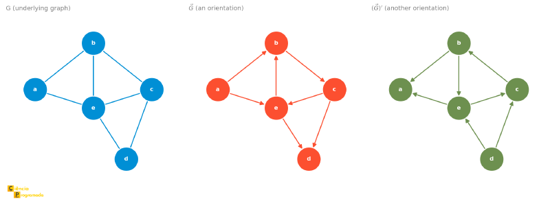
The result is the underlying graph \(G\), with edges \((a,b), (a,e), (b,c), (b,e), (e,c), (c,d), (d,e)\), 7 edges, one fewer than the 8 original arcs of \(D\). The figure below shows the two steps:
An orientation of a graph \(G\) is a digraph \(\vec{G}\) obtained by specifying a direction for each edge of \(G\). The orientation of a graph is not unique: the same \(G\) admits several different orientations.
Example: two different orientations of the same graph
Problem: Find two different orientations of the underlying graph \(G\) from the previous example.
Solution: Two possibilities:
- \(\vec{G}\): \((a,b), (a,e), (b,c), (e,b), (c,e), (c,d), (e,d)\)
- \((\vec{G})^{\prime}\): the opposite orientation of each edge, \((b,a), (e,a), (c,b), (b,e), (e,c), (d,c), (d,e)\)
Both are valid digraphs over the same underlying graph \(G\), but with arcs pointing in different directions, which is why the orientation of a graph is not unique, as the figure shows:
In-Degree and Out-Degree #
In digraphs, each vertex has two degrees:
For a vertex \(v\) in a digraph \(D\):
- In-degree: \(d^-(v) = |\{(u,v) \in E(D)\}|\), the number of arcs arriving at \(v\)
- Out-degree: \(d^+(v) = |\{(v,u) \in E(D)\}|\), the number of arcs leaving \(v\)
Special vertices:
- Source: \(d^-(v) = 0\), that is, no arc arrives at \(v\)
- Sink: \(d^+(v) = 0\), that is, no arc leaves \(v\)
Handshaking-Like Formula #
Proof: Each arc \((u,v)\) contributes 1 to \(d^+(u)\) and 1 to \(d^-(v)\). Summing over all arcs, each sum counts each arc exactly once. Therefore, \(\sum d^-(v) = \sum d^+(v) = |E(D)|\), which is what we wanted to prove. \(\blacksquare\)
Example: degrees in the digraph above
Problem: Compute the in-degree and the out-degree of each vertex of the digraph \(D\) from the example above (\(V = \{a,b,c,d,e\}\)), and identify sources and sinks.
Solution:
| Vertex | \(d^+(v)\) | \(d^-(v)\) |
|---|---|---|
| \(a\) | 2 | 0 |
| \(b\) | 2 | 2 |
| \(c\) | 0 | 3 |
| \(d\) | 2 | 0 |
| \(e\) | 2 | 3 |
\(a\) and \(d\) are sources; \(c\) is a sink.
Sum of the out-degrees: \(2+2+0+2+2 = 8 = |E|\). ✓
Checking with code
Counting arcs by hand works for small digraphs, but networkx already
provides the in-degree and the out-degree as methods of the digraph itself:
D.in_degree(v) and D.out_degree(v). The code below goes through each
vertex, computes both degrees, and marks which one is a source
(\(d^-=0\)) or a sink (\(d^+=0\)):
import networkx as nx

D = nx.DiGraph([("a", "b"), ("b", "c"), ("a", "e"), ("b", "e"),
                ("e", "b"), ("e", "c"), ("d", "c"), ("d", "e")])

for v in sorted(D.nodes()):
    d_plus, d_minus = D.out_degree(v), D.in_degree(v)
    role = " (source)" if d_minus == 0 else " (sink)" if d_plus == 0 else ""
    print(f"{v}: d+={d_plus}, d-={d_minus}{role}")
a: d+=2, d-=0 (source)
b: d+=2, d-=2
c: d+=0, d-=3 (sink)
d: d+=2, d-=0 (source)
e: d+=2, d-=3The result matches the table computed by hand exactly.
Paths and Cycles in Digraphs #
The definitions of walk, trail, path, and cycle, already seen in Paths, Cycles, and Connectivity, still hold, but now with an important restriction: we must follow the directions of the arcs.
A directed walk in a digraph \(D\) is a sequence of vertices \(P = v_0, v_1, \ldots, v_k\) such that \((v_i, v_{i+1}) \in E(D)\) for \(0 \leq i \leq k-1\), that is, each step of the sequence follows an arc of \(D\) in the indicated direction. Vertices and arcs can repeat.
A directed trail is a directed walk in which no arc repeats (but vertices can repeat).
A directed path is a directed walk in which no vertex repeats (and therefore no arc repeats either).
Example: walk, trail, and path in the same digraph
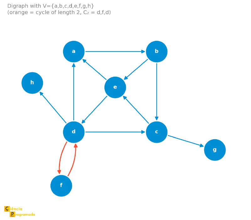
Problem: Consider the digraph with \(V = \{a,b,c,d,e,f,g,h\}\) and arcs \(E = \{(a,b),(b,c),(b,e),(c,e),(c,g),(e,a),(e,d),(d,a),(d,c),(d,f),(f,d),(d,h)\}\), shown in the figure below. Classify the sequences \(P_1 = a,b,c,e,a,b,c,g\), \(P_2 = a,b,e,d,f,d,c,g\), and \(P_3 = a,b,c,g\).
Solution:
- \(P_1\) is a directed walk from \(a\) to \(g\): the arcs \((a,b)\) and \((b,c)\) are traversed twice, so it is not a trail.
- \(P_2\) is a directed trail from \(a\) to \(g\): no arc repeats, but the vertex \(d\) appears twice, so it is not a path.
- \(P_3\) is a directed path from \(a\) to \(g\): no vertex repeats.
In addition, \(C_1 = a,b,c,e,d,a\) is a directed cycle, and \(C_2 = d,f,d\) is a directed cycle of length 2, possible because \((d,f)\) and \((f,d)\) are both arcs of \(D\).
The cycle \(C_2 = d,f,d\) in the example above illustrates a fact exclusive to digraphs: if \((u,v)\) and \((v,u)\) are both arcs, then \(u \to v \to u\) is a cycle of length 2. In simple (undirected) graphs, this does not happen, since the same edge cannot be traversed twice in a cycle.
Reachability: we say that \(v\) reaches \(u\) if there is a directed path from \(v\) to \(u\).
Example: reachability
Problem: In the digraph of the previous figure, which vertices does \(a\) reach? Is there any vertex that does not reach \(a\)?
Solution: \(a\) reaches \(g\) (via \(a,b,c,g\)), reaches \(f\) (via \(a,b,e,d,f\)), and reaches \(h\) (via \(a,b,e,d,h\)); in fact, \(a\) reaches all the other vertices.
This does not hold for every vertex: \(g\) has no arc leaving it, so \(g\) reaches nobody, and in particular, \(g\) does not reach \(a\).
Connectivity in Digraphs #
The notion of connectivity, seen in Paths, Cycles, and Connectivity for ordinary graphs, is richer in digraphs, because directions matter:
\(D\) is strongly connected if for every pair \(v, w \in V\) there is a directed path from \(v\) to \(w\) and from \(w\) to \(v\).
\(D\) is unilaterally connected if for every pair \(v, w \in V\) there is a directed path from \(v\) to \(w\) or from \(w\) to \(v\) (at least one of the two).
\(D\) is weakly connected if the underlying graph is connected (ignoring the directions).
\(D\) is disconnected if the underlying graph is disconnected.
Connectivity Hierarchy #
$$\text{Strongly connected} \implies \text{Unilaterally connected} \implies \text{Weakly connected}$$The implications are strict: each level is weaker, as the following examples show.
Example: strongly connected
Problem: Verify that the digraph \(D\) with \(V=\{a,b,c,d,e\}\) and arcs \(E = \{(a,b),(b,c),(c,d),(d,a),(a,e),(c,e),(e,b),(e,d)\}\), shown below, is strongly connected.
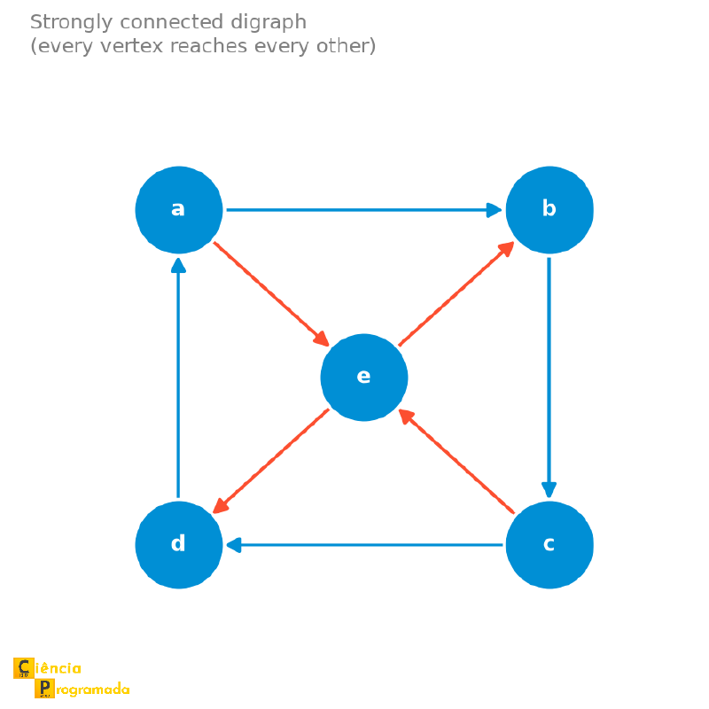
Solution: It suffices to show that, starting from any vertex, we reach all the others. For example, starting from \(a\): we reach \(e\) directly, \(b\) via \(a,b\), \(c\) via \(a,b,c\), and \(d\) via \(a,e,d\) (or \(a,b,c,d\)). Repeating this check from each vertex, we confirm that \(D\) is strongly connected.
Example: the three levels of connectivity side by side
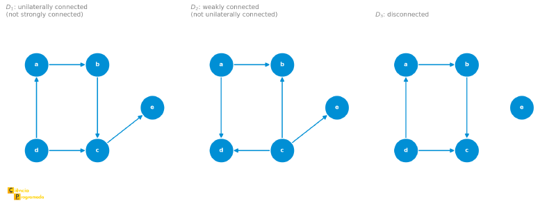
Problem: Classify the three digraphs below, all with \(V = \{a,b,c,d,e\}\), by their level of connectivity:
- \(D_1\): arcs \((a,b), (d,a), (b,c), (d,c), (c,e)\).
- \(D_2\): arcs \((a,b), (a,d), (c,b), (c,d), (c,e)\).
- \(D_3\): arcs \((a,b), (d,a), (b,c), (d,c)\), with \(e\) isolated.
Solution:
- In \(D_1\), \(d\) is a source that reaches all the others (\(d \to a \to b \to c \to e\)), and \(e\) is a sink reached by all the others. Since \(a\), \(b\), and \(c\) form a direct chain \(a \to b \to c\), every pair of vertices has a path in at least one direction, and \(D_1\) is unilaterally connected. But since nothing arrives at \(d\) and \(e\) reaches nobody, \(D_1\) is not strongly connected.
- In \(D_2\), \(a\) only reaches \(b\) and \(d\), while \(c\) reaches \(b\), \(d\), and \(e\): neither reaches the other. This single pair is enough for \(D_2\) not to be unilaterally connected. But the underlying graph is connected (all vertices link up through \(a\) and \(c\)), so \(D_2\) is weakly connected.
- In \(D_3\), the vertex \(e\) is isolated: no arc links it to the others, not even ignoring direction. Since the underlying graph is already disconnected, \(D_3\) is disconnected.
Checking with code
Verifying connectivity by hand requires checking paths between many pairs
of vertices, which is tiresome even in small digraphs. networkx has a
ready-made function for each of the three levels: nx.is_strongly_connected,
nx.is_semiconnected (that is the technical name for “unilaterally
connected”), and nx.is_weakly_connected:
import networkx as nx

D1 = nx.DiGraph([("a", "b"), ("d", "a"), ("b", "c"), ("d", "c"), ("c", "e")])
D2 = nx.DiGraph([("a", "b"), ("a", "d"), ("c", "b"), ("c", "d"), ("c", "e")])
D3 = nx.DiGraph([("a", "b"), ("d", "a"), ("b", "c"), ("d", "c")])
D3.add_node("e")  # e isolated

for name, D in [("D1", D1), ("D2", D2), ("D3", D3)]:
    print(f"{name}: strong={nx.is_strongly_connected(D)}, "
          f"unilateral={nx.is_semiconnected(D)}, "
          f"weak={nx.is_weakly_connected(D)}")
D1: strong=False, unilateral=True, weak=True
D2: strong=False, unilateral=False, weak=True
D3: strong=False, unilateral=False, weak=FalseNote that weak=True for \(D_1\) too: that makes sense, since
unilaterally connected implies weakly connected (the hierarchy seen
before). Only \(D_3\) has weak=False, precisely because \(e\) is
isolated.
A digraph that is not strongly connected splits into strongly connected
components: the largest sets of vertices in which each one reaches all the others.
In the digraph of the walk examples, they are \(\{a,b,c,d,e,f\}\),
\(\{g\}\), and \(\{h\}\). Finding them is a classic problem, solved in
linear time, \(O(n + m)\), by two algorithms based on depth-first search:
Robert Tarjan’s, published in 1972, and S. Rao Kosaraju’s,
described in 1978 and published by Micha Sharir in 1981 (see the entry
Strongly connected component).
In networkx, the function is nx.strongly_connected_components:
import networkx as nx

D = nx.DiGraph([
    ("a", "b"), ("b", "c"), ("b", "e"), ("c", "e"), ("c", "g"), ("e", "a"),
    ("e", "d"), ("d", "a"), ("d", "c"), ("d", "f"), ("f", "d"), ("d", "h"),
])
print(sorted(sorted(c) for c in nx.strongly_connected_components(D)))
# Output: [['a', 'b', 'c', 'd', 'e', 'f'], ['g'], ['h']]
Matrix Representation #
Adjacency Matrix of a Digraph #
For \(D\) with \(V = \{v_1, \ldots, v_n\}\), the adjacency matrix \(A = (a_{ij})\) is \(n \times n\):
$$a_{ij} = \begin{cases} 1 & \text{if } (v_i, v_j) \in E(D) \\ 0 & \text{otherwise} \end{cases}$$The adjacency matrix of a digraph is not symmetric in general, unlike that of undirected graphs.
Relation to degrees:
- Sum of row \(i\): gives \(d^+(v_i)\) (out-degree)
- Sum of column \(j\): gives \(d^-(v_j)\) (in-degree)
Example: adjacency matrix
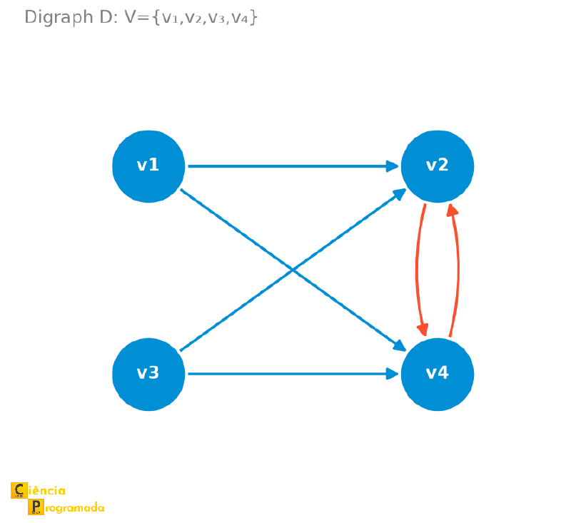
Problem: Build the adjacency matrix of the digraph \(D\) with \(V = \{v_1,v_2,v_3,v_4\}\) and arcs \((v_1,v_2), (v_1,v_4), (v_3,v_2), (v_3,v_4), (v_4,v_2), (v_2,v_4)\), and identify sources and sinks from it.
Solution:
$$A = \begin{array}{c|cccc} & v_1 & v_2 & v_3 & v_4 \\ \hline v_1 & 0 & 1 & 0 & 1 \\ v_2 & 0 & 0 & 0 & 1 \\ v_3 & 0 & 1 & 0 & 1 \\ v_4 & 0 & 1 & 0 & 0 \end{array}$$- Row of \(v_1\): sum = 2 = \(d^+(v_1)\)
- Column of \(v_2\): sum = \(1+0+1+1 = 3 = d^-(v_2)\)
- The columns of \(v_1\) and \(v_3\) are entirely zero: \(v_1\) and \(v_3\) are sources (no arc arrives at them)
- No row is entirely zero: \(D\) has no sink
Incidence Matrix of a Digraph #
For \(D\) with \(n\) vertices and \(m\) arcs, the incidence matrix \(B = (b_{ij})\) is \(n \times m\):
$$b_{ij} = \begin{cases} +1 & \text{if the arc } e_j \text{ diverges from } v_i \text{ (tail)} \\ -1 & \text{if the arc } e_j \text{ converges to } v_i \text{ (head)} \\ 0 & \text{otherwise} \end{cases}$$Each column has exactly one \(+1\) (the tail of the arc) and one \(-1\) (the head of the arc).
Example: incidence matrix
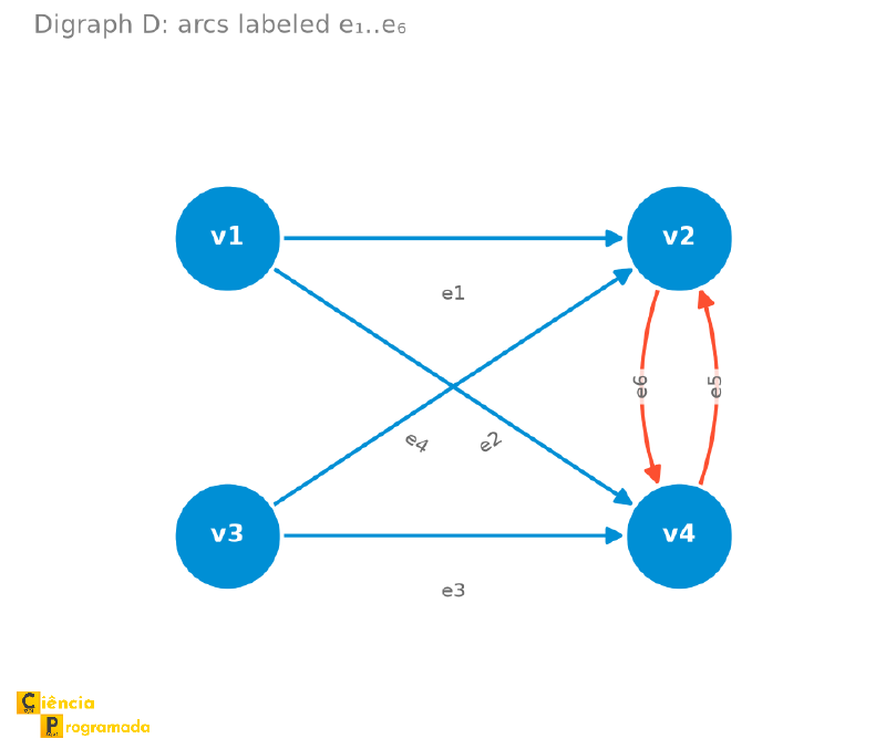
Problem: Build the incidence matrix of the same digraph \(v_1,v_2,v_3,v_4\) from the previous example, now with the arcs labeled \(e_1=(v_1,v_2), e_2=(v_3,v_2), e_3=(v_3,v_4), e_4=(v_1,v_4), e_5=(v_4,v_2), e_6=(v_2,v_4)\):
Solution:
$$B = \begin{array}{c|cccccc} & e_1 & e_2 & e_3 & e_4 & e_5 & e_6 \\ \hline v_1 & 1 & 0 & 0 & 1 & 0 & 0 \\ v_2 & -1 & -1 & 0 & 0 & -1 & 1 \\ v_3 & 0 & 1 & 1 & 0 & 0 & 0 \\ v_4 & 0 & 0 & -1 & -1 & 1 & -1 \end{array}$$Each column has exactly one \(+1\) and one \(-1\): for example, the column of \(e_5\) has \(+1\) at \(v_4\) and \(-1\) at \(v_2\), confirming the arc \((v_4,v_2)\).
Checking with code
networkx computes both matrices out of the box: nx.to_numpy_array for
the adjacency matrix and nx.incidence_matrix for the incidence matrix.
Just one detail: the sign convention of networkx is the opposite of ours
(\(-1\) at the tail and \(+1\) at the head, instead of \(+1\) at the
tail and \(-1\) at the head), so it is enough to multiply the result by
\(-1\) to match the matrix \(B\) we computed by hand:
import networkx as nx

D = nx.DiGraph()
D.add_edges_from([("v1", "v2"), ("v1", "v4"), ("v3", "v2"),
                   ("v3", "v4"), ("v4", "v2"), ("v2", "v4")])
vertices = ["v1", "v2", "v3", "v4"]
arcs = [("v1", "v2"), ("v3", "v2"), ("v3", "v4"), ("v1", "v4"), ("v4", "v2"), ("v2", "v4")]  # e1..e6

A = nx.to_numpy_array(D, nodelist=vertices, dtype=int)
print("Adjacency matrix:\n", A)

B = -nx.incidence_matrix(D, nodelist=vertices, edgelist=arcs, oriented=True).toarray().astype(int)
print("Incidence matrix:\n", B)
Adjacency matrix:
[[0 1 0 1]
[0 0 0 1]
[0 1 0 1]
[0 1 0 0]]
Incidence matrix:
[[ 1 0 0 1 0 0]
[-1 -1 0 0 -1 1]
[ 0 1 1 0 0 0]
[ 0 0 -1 -1 1 -1]]Both match, arc by arc, the matrices \(A\) and \(B\) computed in the examples above.
Applications of Digraphs #
With the theoretical basis established, it is worth highlighting how digraphs show up in practice, often as a central part of other structures:
- Network flow: water in pipes with valves, electric current in circuits; the direction of the flow is part of the model
- The World Wide Web: pages are vertices and hyperlinks are arcs; PageRank (detailed in Graphs: A Language for Modeling Connections) uses the in- and out-degrees of this giant digraph to estimate the relevance of each page
- Call graphs: in software analysis, which functions call which; an arc \((f,g)\) means that \(f\) calls \(g\)
- DAGs (directed acyclic graphs): digraphs with no directed cycle, used to model dependencies
A DAG (Directed Acyclic Graph) is an acyclic digraph (with no directed cycles). It is used in:
- Scheduling tasks with dependencies (the arc \((A, B)\) means “A before B”), as in Apache Airflow
- Installing packages with dependencies (in real managers, such as npm and pip, cycles are tolerated, and the DAG is the ideal case)
- Analyzing dependencies in Makefiles
- Representing genealogies
Topological Sort #
In a DAG of dependencies, the practical question is: in what order should we run the tasks, so that none runs before those it needs? The answer is a topological sort.
A topological sort of a digraph \(D\) is a list of all its vertices in which, for every arc \((u, v)\), \(u\) appears before \(v\).
A digraph admits a topological sort if and only if it is a DAG.
Proof: (\(\Rightarrow\)) Suppose \(D\) has a topological sort and also a directed cycle. Among the vertices of the cycle, let \(v\) be the one that appears first in the sort. The arc of the cycle that arrives at \(v\) leaves from a vertex that appears after \(v\), which the sort forbids. Hence \(D\) has no cycles.
(\(\Leftarrow\)) First, every DAG has a source. If no vertex were a source, we could start from any vertex and always walk backward, along an arc that arrives at the current vertex; since there are finitely many vertices, one would repeat, and the stretch between the two visits would be a directed cycle. Now, by induction on the number of vertices: put a source \(s\) at the start of the list; the digraph \(D - s\) still has no cycles and, by the inductive hypothesis, has a topological sort, which comes after \(s\). No arc arrives at \(s\), so no arc is violated.
Therefore, a digraph admits a topological sort if and only if it is a DAG, which is what we wanted to prove. \(\blacksquare\)
The second half of the proof is already an algorithm, described by Arthur B. Kahn in 1962: remove a source, then another, and so on. To avoid searching for sources from scratch at each step, Kahn’s algorithm keeps the in-degree of each vertex and a queue with the current sources; when removing a vertex \(u\), it decreases by 1 the in-degree of each vertex that \(u\) points to, and any vertex that reaches 0 enters the queue. If the queue empties before all vertices have left, a cycle remains. Each vertex and each arc are handled once: \(O(n + m)\) time (see the entry Topological sorting).
from collections import deque

import networkx as nx

tasks = nx.DiGraph([
    ("extract", "clean"), ("clean", "train"), ("train", "evaluate"),
    ("clean", "plots"), ("evaluate", "report"), ("plots", "report"),
])


def topological_order(D):
    """Kahn's algorithm: a topological sort of D, or None if D has a cycle."""
    in_degree = {v: D.in_degree(v) for v in D}
    queue = deque(v for v in D if in_degree[v] == 0)  # the sources
    order = []
    while queue:
        u = queue.popleft()
        order.append(u)
        for w in D.successors(u):
            in_degree[w] -= 1
            if in_degree[w] == 0:
                queue.append(w)
    return order if len(order) == D.number_of_nodes() else None


print(topological_order(tasks))
# Output: ['extract', 'clean', 'train', 'plots', 'evaluate', 'report']
print(list(nx.topological_sort(tasks)))
# Output: ['extract', 'clean', 'train', 'plots', 'evaluate', 'report']

tasks.add_edge("report", "extract")  # closes a cycle
print(topological_order(tasks))  # None
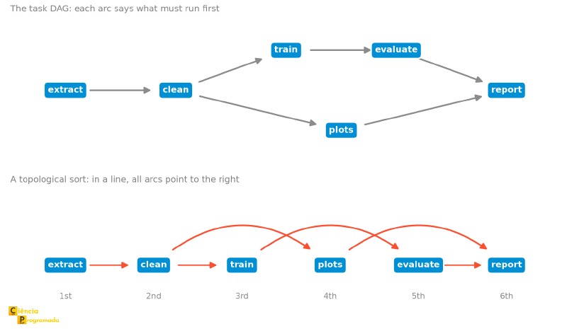
A DAG usually has several topological sorts (here, plots could come before
train), and any of them is a valid order of execution. The figure below
shows the example DAG and, below it, the same vertices in a line, in the order found:
Application: Apache Airflow
Apache Airflow is a tool
for orchestrating data pipelines and models each pipeline literally
as a DAG: each task is a vertex, and the >> operator declares a dependency
arc between two tasks.
from datetime import datetime

from airflow import DAG
from airflow.operators.python import PythonOperator


def extract_data():
    print("extracting the sales data")


def transform_data():
    print("transforming the data")


def load_data():
    print("loading the data into the database")


with DAG("sales_pipeline", start_date=datetime(2026, 1, 1), schedule="@daily") as dag:
    extract = PythonOperator(task_id="extract_data", python_callable=extract_data)
    transform = PythonOperator(task_id="transform_data", python_callable=transform_data)
    load = PythonOperator(task_id="load_data", python_callable=load_data)

    extract >> transform >> load  # DAG arcs: extract -> transform -> load
Translating to the language of this article: each PythonOperator is a
vertex (a task that runs a Python function); the with DAG(...) block declares the digraph itself, with a name and a run
frequency; and the line extract >> transform >> load declares the
arcs \((\text{extract}, \text{transform})\) and \((\text{transform}, \text{load})\),
in the order in which the tasks need to run. At execution time, Airflow follows
a topological sort of this DAG.
If someone tried to close the cycle with load >> extract, Airflow
would reject the DAG at validation: acyclicity is a rule the tool enforces.
Comparison: Graph vs. Digraph #
| Feature | Graph | Digraph |
|---|---|---|
| Edges/Arcs | Unordered pairs \(\{u,v\}\) | Ordered pairs \((u,v)\) |
| Degree | \(d(v)\) (single) | \(d^+(v)\) (out) and \(d^-(v)\) (in) |
| Special vertices | n/a | Source (\(d^- = 0\)), Sink (\(d^+ = 0\)) |
| Adjacency matrix | Symmetric | Not necessarily symmetric |
| Connectivity | Connected / Disconnected | Strong / Unilateral / Weak / Disconnected |
| Handshaking | \(\sum d(v) = 2|E|\) | \(\sum d^+(v) = \sum d^-(v) = |E|\) |
Summary Table #
| Concept | Expression/Definition |
|---|---|
| Digraph | \(D = (V,E)\), with \(E\) made of ordered pairs (arcs) |
| In-degree / out-degree | \(d^-(v) = |\{(u,v) \in E(D)\}|\), \(d^+(v) = |\{(v,u) \in E(D)\}|\) |
| Source / Sink | \(d^-(v) = 0\) (source) / \(d^+(v) = 0\) (sink) |
| Handshaking for digraphs | \(\sum_{v} d^-(v) = \sum_{v} d^+(v) = |E(D)|\) |
| Underlying graph | \(D\) without directions, without parallel edges |
| Orientation | \(\vec{G}\): digraph obtained by choosing a direction for each edge of \(G\) (not unique) |
| Strongly connected | Every pair \(v,w\) has a path from \(v\) to \(w\) and from \(w\) to \(v\) |
| Unilaterally connected | Every pair \(v,w\) has a path from \(v\) to \(w\) or from \(w\) to \(v\) |
| Weakly connected | The underlying graph is connected |
| Disconnected | The underlying graph is disconnected |
| Adjacency matrix | \(a_{ij} = 1\) if \((v_i,v_j) \in E(D)\), \(0\) otherwise |
| Incidence matrix | \(b_{ij} = +1\) (tail), \(-1\) (head), \(0\) otherwise |
| Strongly connected components | Largest sets of mutually reachable vertices; Tarjan and Kosaraju in \(O(n+m)\) |
| Topological sort | Exists \(\iff\) \(D\) is a DAG; Kahn’s algorithm in \(O(n+m)\) |
Exercises #
Exercise 1: Sources and sinks
For the digraph \(D\) with vertices \(\{a,b,c,d\}\) and arcs \(\{(a,b),(a,c),(c,a),(c,b),(d,a),(d,c)\}\):
(a) Which are the sources? (b) Which are the sinks? (c) Does \(a\) reach all vertices? (d) Is \(D\) strongly connected?
Solution
(a) Source: \(d\), since no arc arrives at \(d\) (\(d^-(d) = 0\)).
(b) Sink: \(b\), since no arc leaves \(b\) (\(d^+(b) = 0\)).
(c) From \(a\): \(a \to b\) ✓, \(a \to c\) ✓, but \(a\) does not reach \(d\). False.
(d) No, since \(d\) is a source and no vertex reaches \(d\). Hence \(D\) is not strongly connected.
Exercise 2: Connectivity
Classify as strongly, unilaterally, or weakly connected:
(a) Linear chain \(a \to b \to c \to d \to e \to f\) (b) Cycle \(a \to b \to c \to a\) with extra arc \(b \to d\)
Solution
(a) Unilaterally connected: from \(a\) we reach all vertices. For any pair \((v_i, v_j)\) with \(i < j\), there is a path from \(v_i\) to \(v_j\). But \(f\) does not reach \(a\): it is not strongly connected.
(b) The vertex \(d\) has no arc leaving it, it is a sink and reaches nobody. Since \(d\) does not reach any other vertex, the digraph is not strongly connected. But every vertex reaches \(d\) (\(a \to b \to d\), \(b \to d\), \(c \to a \to b \to d\)), and among \(a\), \(b\), and \(c\) the cycle guarantees a path in both directions, so every pair has a path in at least one direction, and the digraph is unilaterally connected.
Final Series Recap #
With digraphs, we have completed the fundamentals of graph theory. Recapping “The Mathematics of Connections”:
| Article | Central Topic |
|---|---|
| Introduction | History, Königsberg, applications |
| Definitions | \(G=(V,E)\), subgraphs, \(K_n\), cliques |
| Degree | \(d(v)\), regular graphs, Handshaking |
| Isomorphism | Structure-preserving bijections, matrices |
| Paths | Walk/trail/path/cycle, connectivity, BFS and Dijkstra, bipartite |
| Trees | Acyclic+connected, \(m=n-1\), center, spanning |
| Eulerian/Hamiltonian | Special tours, Traveling Salesman Problem (TSP) |
| Planar | Euler’s formula, \(K_5\) and \(K_{3,3}\), Kuratowski, coloring and Four Colors |
| Digraphs | Broken symmetry, oriented degrees, DAGs, topological sort |
This is the last article of the series “The Mathematics of Connections”.


