

In Graphs: A Language for Modeling Connections, we saw that the Seven Bridges of Königsberg problem boils down to a parity argument: the four regions of the city (Altstadt, Kneiphof, Lomse, and Vorstadt) have degrees 3, 5, 3, and 3, respectively. Every region that is neither the start nor the end of a walk must have an even number of bridges; since all four regions of Königsberg have odd degree, the complete walk is impossible.
This informal argument hides two concepts that deserve their own names and a rigorous proof. First: what exactly does “traversing each edge exactly once” mean? A graph that admits this kind of traversal is called an Eulerian graph. Second: what if, instead of crossing every bridge, we only wanted to visit each region exactly once? This question, similar on the surface, is actually a different problem, and a much harder one, which gives rise to Hamiltonian graphs.
In this article, we formalize both concepts, prove Euler’s Theorem, which characterizes Eulerian graphs, and explore why the analogous question about vertices resists a simple characterization to this day, culminating in the Traveling Salesman Problem.
Why do Eulerian and Hamiltonian graphs matter? #
Knowing whether a graph admits these two kinds of traversal is a recurring practical problem in computer science and engineering:
- Urban routing: finding a route that goes through each street of a neighborhood exactly once (garbage collection, mail delivery, snow removal, pipe inspection) is an Eulerian problem. When the graph is not Eulerian and some streets must be repeated, the problem becomes the Chinese Postman Problem, which looks for the shortest total route.
- Bioinformatics: assembling a genome from short DNA fragments is modeled with a De Bruijn graph, in which the assembly corresponds to an Eulerian trail; this idea is behind many short-read assemblers.
- Logistics and deliveries: deciding the order in which to visit a set of addresses while minimizing the distance traveled is the Traveling Salesman Problem, a Hamiltonian question.
- Circuit design: planning the path of a drill or solder probe that must visit each point of a printed circuit board exactly once.
- Task scheduling: sequencing operations on a machine that must go through each configuration of the system exactly once.
The good news is that the Eulerian problem has a simple and efficient solution, as we will see next. The bad news is that the Hamiltonian problem (similar in formulation) is among the hardest that computer science knows.
Two problems, one graph #
To appreciate the difference between the two problems, consider seven cities \(a, b, c, d, e, f, g\) connected by roads, represented by the graph below.
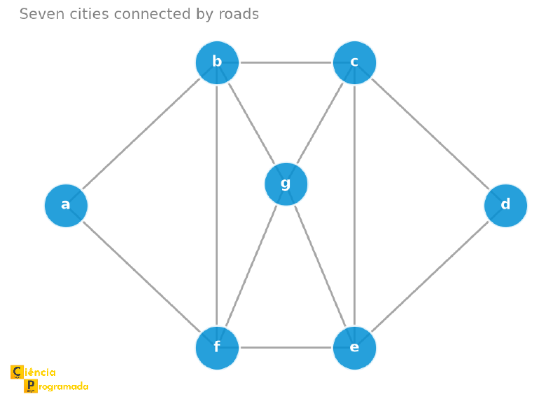
The explorer problem. An explorer wants to travel each road exactly once, starting at \(a\) and returning to \(a\) at the end. A route that solves the problem is \(a \to b \to c \to d \to e \to f \to b \to g \to c \to e \to g \to f \to a\). Notice that the explorer passes through \(b\), \(c\), \(e\), \(f\), and \(g\) more than once; what matters is that each of the 12 roads (edges) of the graph is used exactly once.
The traveler problem. A traveler wants to visit each city exactly once, starting at \(a\) and returning to \(a\) at the end. A route that solves this problem is \(a \to b \to c \to d \to e \to g \to f \to a\). Here the logic is reversed: each city (vertex) appears only once, but not every road (edge) needs to be used; the diagonal \(bg\), for example, is left out.
- The explorer problem is to find a closed trail that includes every edge of the graph.
- The traveler problem is to find a cycle that includes every vertex of the graph.
The first is the Eulerian problem; the second, the Hamiltonian one. We will treat them separately, starting with the simpler one.
Eulerian Graphs #
An Eulerian trail in a graph \(G\) is a trail (with no repeated edges) that includes each edge of \(G\) exactly once. If this trail is closed (starts and ends at the same vertex), we call it an Eulerian circuit.
A connected graph \(G\) is Eulerian if it admits an Eulerian circuit.
Euler’s Theorem #
The informal argument we gave in the opening (each pass through a region uses up a pair of bridges, so only the start and the end can have odd degree) is the easy half of the following theorem. Let us state and prove it precisely.
A connected graph \(G\) is Eulerian if and only if every vertex of \(G\) has even degree.
Proof of the necessary condition (Eulerian → even degrees):
Let \(C\) be an Eulerian circuit of \(G\). Each time \(C\) passes through a vertex \(v\), it “enters” through one edge and “leaves” through another, using up two units of the degree of \(v\) (the starting vertex counts the exit at the beginning and the entry at the end, since the circuit is closed). Since each edge of the graph is used exactly once, the degree of \(v\) equals twice the number of passes of \(C\) through \(v\). Therefore, \(d(v)\) is even for every vertex \(v\) of \(G\), which is what we wanted to prove. \(\blacksquare\)
Proof of the sufficient condition (even degrees → Eulerian): by strong induction on the number \(m\) of edges. Suppose that every connected graph with even degrees, at least one edge, and fewer than \(m\) edges is Eulerian, and let \(G\) be a connected graph with \(m\) edges (\(m \geq 1\)) and all degrees even.
Step 1: \(G\) has a cycle. Since \(G\) is connected and has edges, every vertex has degree at least 1; since the degrees are even, every vertex has degree at least 2. Take a path \(P = v_0, v_1, \ldots, v_k\) of maximum length in \(G\). The vertex \(v_k\) has at least two neighbors: one is \(v_{k-1}\), and the other, \(w\), must be in \(P\). If it were not, we could extend \(P\) to \(w\), and \(P\) would not be maximum. If \(w = v_i\), then \(v_i, v_{i+1}, \ldots, v_k, v_i\) is a cycle \(C\).
Step 2: remove the cycle. Let \(H\) be the graph obtained by removing from \(G\) the edges of \(C\), without removing vertices. Each vertex of \(C\) loses exactly 2 from its degree, and the others lose nothing: all degrees of \(H\) remain even. \(H\) may be disconnected, but each connected component of \(H\) is a connected graph, with even degrees and fewer than \(m\) edges. By the inductive hypothesis, each component that has edges admits an Eulerian circuit.
Step 3: stitch the circuits together. Every component of \(H\) with edges touches \(C\). Indeed, since \(G\) is connected, there is a path in \(G\) from a vertex of that component to \(C\); the first edge of that path that is not in \(H\) is an edge of \(C\), and the vertex where it starts belongs to both the component and \(C\). Now walk along \(C\): upon first arriving at a vertex of \(C\) where there is still an unvisited component of \(H\), take a detour along the Eulerian circuit of that component, which starts and ends at that vertex, and then continue along \(C\). The result is a closed trail that uses each edge of \(C\) and each edge of \(H\) exactly once, that is, each edge of \(G\) exactly once. (No separate base case is needed: if \(H\) has no edges, the circuit is just \(C\) itself.)
Therefore, \(G\) is Eulerian; together with the necessary condition, a connected graph is Eulerian if and only if all its vertices have even degree, which is what we wanted to prove. \(\blacksquare\)
The theorem and both proofs also hold for multigraphs, counting each loop twice in the degree. The only difference is in Step 1: the “cycle” found may be a loop, or two parallel edges between the same two vertices. It is in this form that Euler’s Theorem is used in the Christofides-Serdyukov algorithm, later on.
This theorem is remarkable because it gives an efficient way to decide whether a graph is Eulerian: just check the parity of the degree of each vertex, without having to actually look for the circuit.
Example: when graphs stop being Eulerian #
Consider the four graphs below, all on subsets of the vertices \(a, b, c, d, e, f, g\); the first reuses the seven-city graph we saw in the motivation. The following figure shows the four side by side.
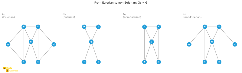
\(G_1\): the seven-city graph
Statement: \(G_1\) is the seven-city graph itself, with vertices \(a, b, c, d, e, f, g\). Is it Eulerian?
Solution: Degrees: \(d(a) = d(d) = 2\); \(d(b) = d(c) = d(e) = d(f) = d(g) = 4\). All degrees are even, so, by Euler’s Theorem, \(G_1\) is Eulerian.
\(G_2\): two triangular “wings” sharing a vertex
Statement: Vertices \(b, c, e, f, g\); edges \(bc, bg, cg, ef, eg, fg\), two triangles, \(bcg\) and \(efg\), sharing the vertex \(g\). Is \(G_2\) Eulerian?
Solution: Degrees: \(d(b) = d(c) = d(e) = d(f) = 2\); \(d(g) = 4\). All even, so \(G_2\) is Eulerian. One possible circuit is \(b \to c \to g \to f \to e \to g \to b\); notice that \(g\) is visited twice, which is perfectly valid in an Eulerian circuit, which does not repeat edges but may repeat vertices.
\(G_3\): a square with both diagonals
Statement: Vertices \(b, c, e, f, g\); edges \(bc, ce, ef, fb, bg, cg, eg, fg\). Is \(G_3\) Eulerian?
Solution: Degrees: \(d(b) = d(c) = d(e) = d(f) = 3\); \(d(g) = 4\). Four vertices of odd degree: \(G_3\) is not Eulerian.
\(G_4\): the square of \(G_3\) with two pendant vertices
Statement: Vertices \(a, b, c, d, e, f, g\); the same edges as \(G_3\), plus \(ab\) and \(cd\). Is \(G_4\) Eulerian?
Solution: Degrees: \(d(a) = d(d) = 1\); \(d(b) = d(c) = d(g) = 4\); \(d(e) = d(f) = 3\). Four vertices of odd degree (\(a\), \(d\), \(e\), \(f\)): \(G_4\) is not Eulerian.
Checking with code
Checking the parity of the degrees by hand works well for small graphs, but
networkx already ships this check in nx.is_eulerian, and can even find
an explicit Eulerian circuit with nx.eulerian_circuit, which implements
Hierholzer’s algorithm:
import networkx as nx

G1 = nx.Graph([("a", "b"), ("a", "f"), ("b", "c"), ("b", "f"), ("b", "g"),
               ("c", "d"), ("c", "e"), ("c", "g"), ("d", "e"), ("e", "f"),
               ("e", "g"), ("f", "g")])
G2 = nx.Graph([("b", "c"), ("b", "g"), ("c", "g"), ("e", "f"), ("e", "g"), ("f", "g")])
G3 = nx.Graph([("b", "c"), ("c", "e"), ("e", "f"), ("f", "b"),
               ("b", "g"), ("c", "g"), ("e", "g"), ("f", "g")])
G4 = nx.Graph([("b", "c"), ("c", "e"), ("e", "f"), ("f", "b"), ("a", "b"),
               ("b", "g"), ("c", "g"), ("e", "g"), ("f", "g"), ("c", "d")])

for name, G in [("G1", G1), ("G2", G2), ("G3", G3), ("G4", G4)]:
    print(f"Is {name} Eulerian? {nx.is_eulerian(G)}")

print("Eulerian circuit of G1:", list(nx.eulerian_circuit(G1, source="a")))
Is G1 Eulerian? True
Is G2 Eulerian? True
Is G3 Eulerian? False
Is G4 Eulerian? False
Eulerian circuit of G1: [('a', 'f'), ('f', 'g'), ('g', 'e'), ('e', 'c'), ('c', 'g'), ('g', 'b'), ('b', 'f'), ('f', 'e'), ('e', 'd'), ('d', 'c'), ('c', 'b'), ('b', 'a')]The result confirms exactly the analysis we did by hand. The circuit found for \(G_1\) is just one among several possible; notice that it passes through \(g\) twice, which is valid, since the only requirement is not to repeat edges.
Open Eulerian trails #
Not every graph with an Eulerian trail needs it to be closed. By relaxing the requirement of returning to the starting point, we arrive at an open version of the theorem, exactly the generalization we promised in Graphs: A Language for Modeling Connections, the article that introduced the Bridges of Königsberg problem and gave rise to all of graph theory.
A connected graph admits an open Eulerian trail (one that starts and ends at distinct vertices) if and only if it has exactly two vertices of odd degree. The trail starts at one of these two vertices and ends at the other.
It is worth quickly recalling the original problem, even for those who have not read the first article of the series: four regions of Königsberg (Altstadt, Kneiphof, Lomse, and Vorstadt), connected by seven bridges over the Pregel River, and the question was whether one could cross each bridge exactly once. The map below shows the layout of the bridges:

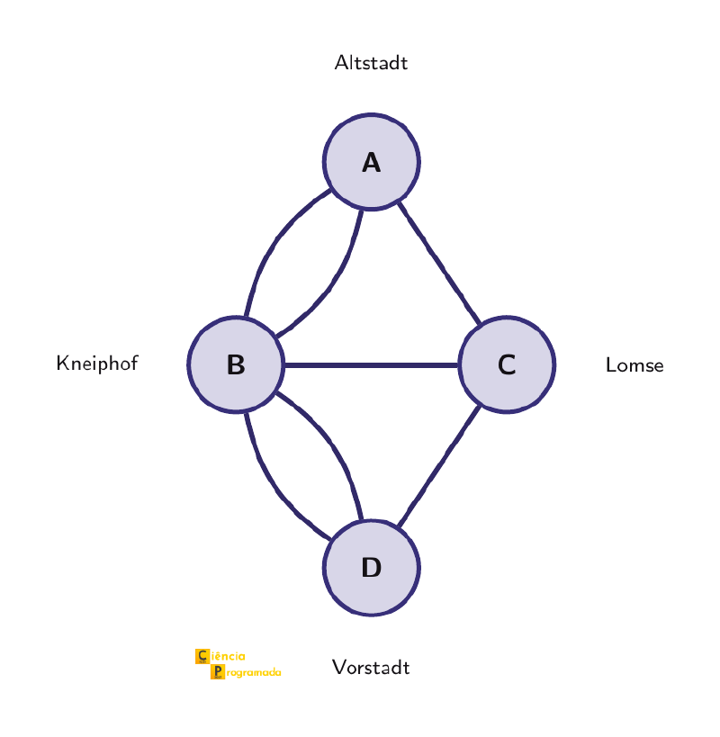
Euler abstracted this map into the graph below: each region became a vertex, each bridge an edge, and the double edges between A-B and B-D represent the pairs of bridges that existed between those regions.
Applying it to Königsberg
The same four odd degrees of Königsberg that we saw in the opening are enough to conclude more than we already knew: since there are four vertices of odd degree (more than two), Königsberg admits neither a closed Eulerian circuit (Euler’s Theorem) nor an open Eulerian trail (this theorem). The answer to the original challenge is, therefore, a definitive no, whatever starting or ending point is chosen.
Hamiltonian Graphs #
A Hamiltonian cycle in \(G\) is a cycle that includes each vertex of \(G\) exactly once. A graph \(G\) is Hamiltonian if it contains a Hamiltonian cycle.
- Eulerian: traverses each edge exactly once (may repeat vertices).
- Hamiltonian: traverses each vertex exactly once (may leave edges out).
Hamilton and the Icosian Game #
The name “Hamiltonian” comes from Sir William Rowan Hamilton (1805-1865), who popularized the problem with the Icosian Game, a puzzle presented in 1857 and sold from 1859. The board represents the graph of a dodecahedron (20 vertices, 30 edges, each vertex with exactly 3 neighbors) and the challenge is: given an initial sequence of five consecutive vertices of a route, complete a cycle that visits the remaining 15 vertices exactly once and returns to the start. The figure below shows the graph drawn as an outer pentagon, a band of 10 vertices, and an inner pentagon (the classic layout used on the original board), with the 5 initial vertices of the challenge in green and a complete Hamiltonian cycle highlighted in orange.
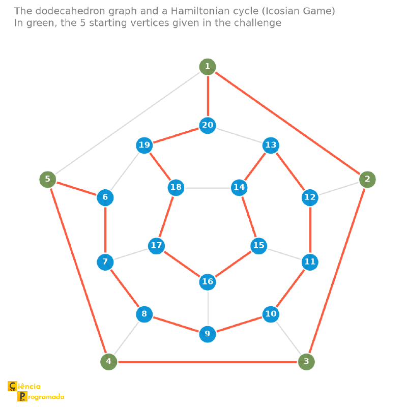
Despite the name, the game’s graph is that of the dodecahedron, not of the icosahedron. The prefix comes from the Greek for “twenty”: the dodecahedron has 20 vertices, and a cycle that goes through all of them has 20 edges.
Not every question has an easy answer #
Unlike the Eulerian problem, deciding whether a graph is Hamiltonian seems, at first sight, a similar question, but no complete and efficient characterization like Euler’s Theorem is known. Deciding whether an arbitrary graph is Hamiltonian is, in fact, an NP-complete problem (the acronym stands for Nondeterministic Polynomial time and identifies the class of the hardest decision problems among those verifiable in polynomial time): no efficient algorithm is known that solves the general case. What exist are partial conditions: sufficient, but not necessary.
A simple observation helps build intuition: the more edges a graph has, the greater the chance that it is Hamiltonian. The cycle \(C_n\) (with \(n\) vertices) is already, trivially, Hamiltonian: it is itself the Hamiltonian cycle. If we add edges to \(C_n\), the resulting graph still contains that same cycle as a subgraph, so it remains Hamiltonian. In the limit, the complete graph \(K_n\), which has all possible edges, is also Hamiltonian. The sequence of figures below illustrates this progression.
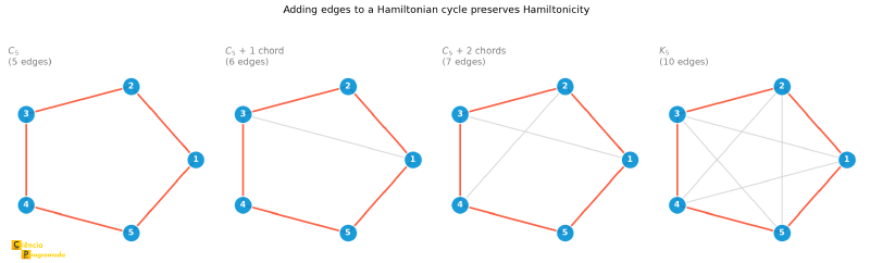
This observation is not a proof, only an intuition that “dense” graphs (with many edges) tend to be Hamiltonian. But it motivates exactly the two most important sufficient-condition theorems of the theory, published a few years apart.
Sufficient Conditions: Dirac and Ore #
If \(G\) has \(n \geq 3\) vertices and \(d(v) \geq \dfrac{n}{2}\) for every \(v \in V(G)\), then \(G\) is Hamiltonian.
If \(G\) has \(n \geq 3\) vertices and \(d(v) + d(w) \geq n\) for every pair of nonadjacent vertices \(v, w\), then \(G\) is Hamiltonian.
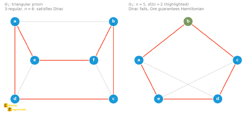
Note that Dirac’s Theorem is a special case of Ore’s: if \(d(v) \geq n/2\) and \(d(w) \geq n/2\) for any \(v, w\), then \(d(v) + d(w) \geq n\) even when \(v\) and \(w\) are not adjacent. Ore’s is, therefore, a strictly broader condition. The two graphs below show a case where Dirac already settles the question and another where only Ore does.
Example: the triangular prism satisfies Dirac
Statement: The graph \(G_1\) has 6 vertices \(a, b, c, d, e, f\) with edges \(ab, ad, ae, bc, bf, cd, cf, de, ef\), a triangular prism: two triangles, \(ade\) and \(bcf\), joined by the three edges \(ab\), \(cd\), and \(ef\). Is \(G_1\) Hamiltonian?
Solution: \(G_1\) is 3-regular: \(d(v) = 3\) for every vertex. Since \(n = 6\), we have \(n/2 = 3\), so \(d(v) = 3 \geq 3 = n/2\) for every \(v\). By Dirac’s Theorem, \(G_1\) is Hamiltonian; indeed, \(a \to d \to c \to b \to f \to e \to a\) is a valid Hamiltonian cycle.
Example: when Dirac fails but Ore works
Statement: The graph \(G_2\) has vertices \(a, b, c, d, e\) and edges \(ab, bc, ae, ad, ce, cd, ed\). Is \(G_2\) Hamiltonian?
Solution: Degrees: \(d(b) = 2\); \(d(a) = d(c) = d(d) = d(e) = 3\). Since \(n = 5\), Dirac’s condition requires degree \(\geq 2.5\) for every vertex, but \(d(b) = 2 < 2.5\). Dirac’s Theorem does not apply.
Testing Ore on the three pairs of nonadjacent vertices (\(a,c\)), (\(b,d\)), and (\(b,e\)):
- \(d(a) + d(c) = 3 + 3 = 6 \geq 5\) ✓
- \(d(b) + d(d) = 2 + 3 = 5 \geq 5\) ✓
- \(d(b) + d(e) = 2 + 3 = 5 \geq 5\) ✓
All nonadjacent pairs satisfy the condition: by Ore’s Theorem, \(G_2\) is Hamiltonian, even though Dirac guarantees nothing. An explicit Hamiltonian cycle: \(a \to b \to c \to d \to e \to a\). This example shows Ore being strictly stronger (broader) than Dirac.
There are Hamiltonian graphs that satisfy neither Dirac nor Ore. The cycle \(C_5\) is Hamiltonian (it is itself the Hamiltonian cycle), but \(d(v) = 2\) for every vertex.
- Dirac: it would need \(d(v) \geq n/2 = 2.5\); we have only \(d(v) = 2\). Fails.
- Ore: every pair of nonadjacent vertices in \(C_5\) has \(d(v) + d(w) = 2 + 2 = 4 < 5 = n\). Fails too.
Both conditions are only sufficient: their absence does not allow us to conclude anything about Hamiltonicity.
The Traveling Salesman Problem (TSP) #
The Traveling Salesman Problem (TSP) is one of the most famous questions in mathematics and computer science:
Given a weighted graph (each edge with a weight, representing distance or cost), find the Hamiltonian cycle of minimum total cost.
A bit of history #
The problem is older than it looks. A German manual from 1832 for traveling salesmen already mentioned the importance of planning the route well, with no mathematical treatment. Mathematics entered the scene still in the 19th century, with William Rowan Hamilton and Thomas Kirkman, who studied cycles that visit each vertex of a graph, the same concept that motivated the Icosian Game we saw earlier. The general form of the problem appeared in the 1930s: the Austrian mathematician Karl Menger, then in Vienna and later at Harvard, studied it under the name Botenproblem (“messenger problem”). The name “traveling salesman problem” first appears in a 1949 report by the mathematician Julia Robinson for the RAND Corporation.
The first major practical breakthrough came in 1954: George Dantzig, Delbert Fulkerson, and Selmer Johnson optimally solved an instance with 49 cities using a cutting-plane method, the seed of the combinatorial optimization techniques used to this day.
A small example #
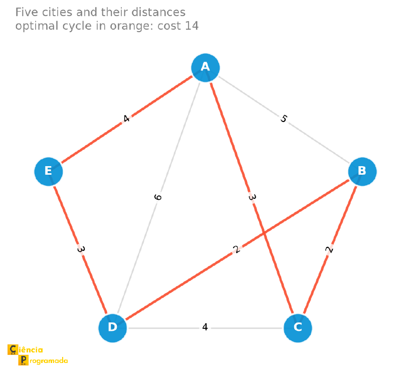
Consider five cities \(A, B, C, D, E\) connected by the roads and distances of the graph below.
Two possible Hamiltonian cycles:
- \(C_1: A \to B \to C \to D \to E \to A\), with cost \(5+2+4+3+4 = 18\)
- \(C_2: A \to C \to B \to D \to E \to A\), with cost \(3+2+2+3+4 = 14\)
Testing all possible Hamiltonian cycles of this graph, \(C_2\) is indeed the one with minimum cost, the optimal solution of this small example.
Why it is hard #
With \(n\) cities, starting from a fixed city, the number of Hamiltonian cycles we can form (counting the two directions of travel as different) is \((n-1)!\):
- 10 cities: \(9! = 362{,}880\) routes
- 20 cities: \(19! \approx 1.22 \times 10^{17}\) routes
- 50 cities: checking by brute force would take longer than the age of the universe
(Since traversing a cycle in one direction or the other gives exactly the same total cost, some authors divide this number by 2 to count only distinct cycles. The order of magnitude of the problem does not change.)
The animation below shows brute force exhaustively testing the cycles of a 7-city TSP until it finds the optimum:

It is worth being precise about what exactly is hard here. The decision version of the problem (“is there a Hamiltonian cycle of cost at most \(k\)?”) is NP-complete. The optimization version (“what is the minimum-cost cycle?”, which is the one we really care about) is NP-hard: at least as hard as any problem in NP. In 1972, Richard Karp proved that deciding whether a graph has a Hamiltonian cycle (the problem we studied in this very article) is NP-complete. That is where the difficulty of the TSP comes from: giving weight 1 to the edges of a graph with \(n\) vertices and weight 2 to the pairs of vertices that are not edges, the graph has a Hamiltonian cycle if and only if the TSP has a cycle of cost \(n\), one more link between the two central themes of this text.
Exact algorithms: beyond brute force #
Brute force is not the only exact option. The Held-Karp algorithm (1962) uses dynamic programming to solve the TSP in \(O(n^2 2^n)\) time, still exponential, but much better than \(O(n!)\):
| \(n\) | \((n-1)!\) (brute force) | \(n^2 2^n\) (Held-Karp) |
|---|---|---|
| 10 | 362,880 | 102,400 |
| 20 | \(1.22 \times 10^{17}\) | \(4.19 \times 10^{8}\) |
| 30 | \(8.84 \times 10^{30}\) | \(9.66 \times 10^{11}\) |
The idea: for each subset \(S\) of cities already visited and each city \(j \in S\), we store the minimum cost to reach \(j\) having visited exactly the cities in \(S\). Each new subset is built from smaller subsets, avoiding recomputing the same partial path several times, the hallmark of any dynamic programming.
The code below implements Held-Karp for our five-city example (using a bitmask to represent subsets of cities, in which bit \(j\) of an integer indicates whether city \(j\) has already been visited):
import math
from itertools import combinations

cities = ["A", "B", "C", "D", "E"]
INF = math.inf
dist = {
    ("A", "B"): 5, ("A", "C"): 3, ("A", "D"): 6, ("A", "E"): 4,
    ("B", "C"): 2, ("B", "D"): 2,
    ("C", "D"): 4,
    ("D", "E"): 3,
}

def d(i, j):
    if i == j:
        return 0
    return dist.get((i, j), dist.get((j, i), INF))

n = len(cities)
# dp[(subset, j)] = minimum cost to visit exactly `subset`
# (bitmask over cities 1..n-1), ending at city j
dp = {}
for j in range(1, n):
    dp[(1 << j, j)] = d(cities[0], cities[j])

for size in range(2, n):
    for subset in combinations(range(1, n), size):
        bits = sum(1 << b for b in subset)
        for j in subset:
            bits_without_j = bits & ~(1 << j)
            dp[(bits, j)] = min(
                dp[(bits_without_j, k)] + d(cities[k], cities[j])
                for k in subset if k != j
            )

all_cities = sum(1 << b for b in range(1, n))
optimal_cost = min(dp[(all_cities, j)] + d(cities[j], cities[0]) for j in range(1, n))
print(f"Optimal cycle cost: {optimal_cost}")
Optimal cycle cost: 14The result matches exactly the \(C_2\) we found by inspection. The difference is that Held-Karp finds this value systematically, without having to enumerate the cycles manually, and keeps working (in principle) for larger instances, although \(2^n\) still grows too fast to be practical beyond about 20-30 cities.
For larger instances, the method of choice is branch-and-bound combined with linear programming techniques (branch-and-cut), which discards whole branches of the search tree whenever it can prove that they do not lead to a solution better than the best one known. The animation below shows the same 7-city TSP solved this way, exploring far fewer branches than brute force:

It is this family of techniques (refined over decades in the Concorde TSP Solver software) that made it possible to optimally solve huge real instances: 15,112 cities in Germany in 2001, 24,978 cities in Sweden in 2004, and a record of 85,900 points (a drilling problem for printed circuit boards) in 2006, using more than 136 CPU-years of processing.
Heuristics: good solutions, quickly #
When the exact approach is too expensive, heuristics find good (not necessarily optimal) solutions in much less time.
The simplest is nearest neighbor: start at any city and, at each step, go to the nearest unvisited city. See below this heuristic in action on a 7-city TSP:

import math

cities = ["A", "B", "C", "D", "E"]
INF = math.inf
dist = {
    ("A", "B"): 5, ("A", "C"): 3, ("A", "D"): 6, ("A", "E"): 4,
    ("B", "C"): 2, ("B", "D"): 2,
    ("C", "D"): 4,
    ("D", "E"): 3,
}


def d(i, j):
    if i == j:
        return 0
    return dist.get((i, j), dist.get((j, i), INF))


def nearest_neighbor(start):
    unvisited = set(cities) - {start}
    tour = [start]
    current = start
    total_cost = 0
    while unvisited:
        # distance tie: the first city in alphabetical order stays
        next_city = min(sorted(unvisited), key=lambda c: d(current, c))
        total_cost += d(current, next_city)
        tour.append(next_city)
        unvisited.remove(next_city)
        current = next_city
    total_cost += d(current, start)
    tour.append(start)
    return tour, total_cost

for city in cities:
    tour, cost = nearest_neighbor(city)
    print(f"{' -> '.join(tour)}: cost {cost}")
A -> C -> B -> D -> E -> A: cost 14
B -> C -> A -> E -> D -> B: cost 14
C -> B -> D -> E -> A -> C: cost 14
D -> B -> C -> A -> E -> D: cost 14
E -> D -> B -> C -> A -> E: cost 14Starting from B, cities C and D are at the same distance (2), and the code breaks the tie by alphabetical order: it goes to C. With another tiebreaking criterion, the route would come out different, and that is how it is with the heuristic in general: the result depends on how ties are broken.
In this small example, nearest neighbor finds the optimum (14) from any starting city, but this is a coincidence of the reduced example, not a general guarantee. On larger instances, this heuristic typically produces tours about 25% longer than the optimum, and in the worst case it can be arbitrarily worse. Still, its simplicity makes it a good starting point for more refined heuristics.
One such improvement is 2-opt: given any tour, look for two edges that, if swapped (undoing a crossing), reduce the total distance. Repeat until no more improvements are found. The figure below shows one such swap:

Applied repeatedly on an initial solution (such as the one from nearest neighbor), 2-opt usually improves the tour considerably: on Euclidean instances, it gives on average solutions about 5% better than those of the Christofides-Serdyukov algorithm, which we will see next, and more sophisticated variants, such as 3-opt and the Lin-Kernighan heuristic, get even closer to the optimum.
The Christofides-Serdyukov algorithm: Eulerian and Hamiltonian together #
No heuristic illustrates the connection between the two themes of this article better than the Christofides-Serdyukov algorithm (1976). It works on metric graphs (where the distances satisfy the triangle inequality) and guarantees a tour with cost at most 1.5 times the optimum. For decades, nobody got a better guarantee. In 2011 came a tiny improvement, but only for a particular case, the graphic TSP (in which the distance between two cities is the number of edges of the shortest path in an unweighted graph); for the general metric TSP, the factor 1.5 was only beaten in 2020, by Anna Karlin, Nathan Klein, and Shayan Oveis Gharan, with a randomized algorithm of factor \(1.5 - 10^{-36}\) (see the entry Christofides algorithm).
The steps of the algorithm use, in sequence, a minimum spanning tree, a minimum-weight matching, and, here is the connection, an Eulerian circuit:
-
1
Minimum spanning tree
Build the minimum spanning tree of the weighted graph. -
2
Matching on the odd-degree vertices
In the minimum spanning tree, identify the vertices of odd degree. By the Handshaking Lemma, this set always has an even number of vertices, which makes it possible to pair them up. Compute the minimum-weight matching among them and add these edges to the tree. -
3
Eulerian circuit
Each odd-degree vertex identified in the previous step had its degree increased by exactly 1 by the matching, and therefore every vertex of the resulting multigraph (tree plus matching) now has even degree. By Euler’s Theorem that we proved in this article, in the version for multigraphs, this multigraph is Eulerian: find an Eulerian circuit in it. -
4
Shortcut to a Hamiltonian cycle
Traverse the Eulerian circuit in the order found, but skip any city already visited, going straight to the next new city. Since the graph is metric, “cutting corners” this way never increases the total cost (triangle inequality). The result is a Hamiltonian cycle, the answer of the algorithm.
The figure below illustrates step 2, the matching of the odd-degree vertices:

And this one shows the shortcut of step 4, which turns the Eulerian circuit into a Hamiltonian cycle:

Checking with code
networkx already implements the four steps above ready to use, in
nx.approximation.christofides. The only requirement is that the graph be
complete. Since our five-city example does not have the edges \(EB\) and
\(EC\), we complete the graph with the metric closure computed by hand
(the shortest possible distance between these pairs going through other
cities): \(d(E,B) = d(E,D) + d(D,B) = 3 + 2 = 5\) and
\(d(E,C) = d(E,A) + d(A,C) = 4 + 3 = 7\).
import networkx as nx

G_complete = nx.Graph()
G_complete.add_weighted_edges_from([
    ("A", "B", 5), ("A", "C", 3), ("A", "D", 6), ("A", "E", 4),
    ("B", "C", 2), ("B", "D", 2), ("B", "E", 5),
    ("C", "D", 4), ("C", "E", 7),
    ("D", "E", 3),
])

tour = nx.approximation.christofides(G_complete, weight="weight")
cost = sum(G_complete[tour[i]][tour[i + 1]]["weight"] for i in range(len(tour) - 1))
print("Tour:", " -> ".join(tour))
print("Cost:", cost)
Tour: A -> E -> D -> B -> C -> A
Cost: 14In this small example, Christofides-Serdyukov finds the optimum itself (14), the same value as \(C_2\), only traversed in the opposite direction. This is not guaranteed in general: the 1.5x guarantee is a worst-case bound, not a typical prediction. On larger, more irregular instances, the algorithm usually delivers tours much closer to the optimum than this theoretical bound suggests.
In other words: Christofides-Serdyukov deliberately builds an Eulerian graph just to “shortcut” it into a Hamiltonian graph, using the two theorems that are the subject of this article as tools of a real approximation algorithm, still used today.
Other popular metaheuristics, such as genetic algorithms, simulated annealing, tabu search, and ant colony optimization (which simulates ants depositing pheromone on the shortest paths), also produce good practical results, but without the mathematical 1.5x guarantee that Christofides-Serdyukov offers for metric graphs.
Special cases #
Not every TSP is equally hard in practice:
- Metric TSP: when the distances satisfy the triangle inequality (\(d(u,w) \leq d(u,v) + d(v,w)\) for any \(u, v, w\)), the most common case in real applications, since geographic distances behave this way. It is what enables the 1.5x guarantee of Christofides-Serdyukov.
- Euclidean TSP: when the cities are points in the plane and the distance is the usual Euclidean distance. It remains NP-hard, but admits a PTAS (polynomial-time approximation scheme) discovered by Sanjeev Arora and Joseph Mitchell (work awarded the 2010 Gödel Prize), which comes as close to the optimum as desired, in polynomial time for any fixed precision.
These special cases explain why the TSP, although NP-hard in general, is routinely solved in practice: most real applications fall into one of these more tractable cases.
Real applications:
- Logistics and delivery routing
- Printed circuit board design (minimizing the soldering probe path)
- Sequencing of operations on industrial machines
- Route planning for robots in automated warehouses
- DNA sequencing in bioinformatics
- Telescope positioning in astronomical surveys
For the complete mathematical treatment, including asymmetric variants, integer linear programming formulations, and the most recent computational records, it is worth consulting the Wikipedia article on the TSP.
Summary #
| Result | Statement |
|---|---|
| Euler’s Theorem | connected \(G\) is Eulerian \(\Leftrightarrow\) every vertex has even degree |
| Open Eulerian Trail | connected \(G\) admits an open Eulerian trail \(\Leftrightarrow\) exactly 2 vertices of odd degree |
| Dirac’s Theorem | \(d(v) \geq n/2\) for all \(v\) \(\Rightarrow\) \(G\) is Hamiltonian |
| Ore’s Theorem | \(d(v)+d(w) \geq n\) for every nonadjacent pair \(\Rightarrow\) \(G\) is Hamiltonian |
| Traveling Salesman Problem | find, among the Hamiltonian cycles of a weighted graph, the one with minimum total cost |
| Christofides-Serdyukov | on metric graphs, builds an Eulerian circuit (minimum spanning tree + matching) and shortcuts it into a Hamiltonian cycle of cost \(\leq 1.5\) times the optimum |
| Counting Hamiltonian cycles | with \(n\) cities, there are \((n-1)!\) possible routes (brute force); Held-Karp solves it in \(O(n^2 2^n)\) |
Comparison: Eulerian vs. Hamiltonian #
| Property | Eulerian | Hamiltonian |
|---|---|---|
| Traverses | All edges | All vertices |
| Exact criterion | Yes: all degrees even | No general criterion exists |
| Open version | Exactly 2 odd degrees | - |
| Sufficient condition | - | Dirac or Ore |
| Verification complexity | \(O(n + m)\) (degrees and connectivity) | NP-complete |
| Optimization version | - | TSP (NP-hard) |
Exercises #
Exercise 1: Eulerian or not?
Determine whether the following graphs are Eulerian, have an open Eulerian trail, or neither:
(a) \(K_5\) (b) \(K_6\) (c) \(K_{3,3}\) (d) \(C_7\)
Solutions
(a) \(K_5\): all 5 vertices have degree 4 (even). Eulerian. ✓
(b) \(K_6\): all 6 vertices have degree 5 (odd). There are 6 vertices of odd degree. No Eulerian trail (neither open nor closed).
(c) \(K_{3,3}\): in complete bipartite graphs \(K_{p,q}\), each vertex in \(X\) has degree \(q\) and each vertex in \(Y\) has degree \(p\). In \(K_{3,3}\): all have degree 3 (odd). There are 6 vertices of odd degree. No Eulerian trail.
(d) \(C_7\): 2-regular graph (all degrees even). Eulerian. The cycle itself is the Eulerian circuit.
Exercise 2: Applying Dirac
Is the graph \(K_4\) (4 vertices, all with degree 3) Hamiltonian? Apply Dirac’s Theorem.
Solution
For \(n = 4\), Dirac’s condition requires \(d(v) \geq n/2 = 2\). Since \(d(v) = 3 \geq 2\) for every \(v\), Dirac’s Theorem confirms that \(K_4\) is Hamiltonian. ✓ (In fact, any ordering of the 4 vertices forms a Hamiltonian cycle in \(K_4\).)
Exercise 3: The Icosian Game challenge
In the dodecahedron graph (20 vertices, each with exactly 3 neighbors, numbered 1 to 20 in the Icosian Game figure above), vertices \(1\) to \(5\) are exactly the outer pentagon of the drawing. A Hamiltonian cycle starts with the sequence \(1 \to 2 \to 3 \to 4 \to 5\). Complete this cycle by going through the remaining 15 vertices. Then, try to find a second solution, different from the first, that also starts with \(1,2,3,4,5\).
Solution
A first solution simply follows the numbering in order: \(1 \to 2 \to 3 \to \cdots \to 19 \to 20 \to 1\).
A second solution, distinct from the first but with the same beginning, is: \(1 \to 2 \to 3 \to 4 \to 5 \to 6 \to 19 \to 18 \to 14 \to 15 \to 16 \to 17 \to 7 \to 8 \to 9 \to 10 \to 11 \to 12 \to 13 \to 20 \to 1\).
Both use the same first five vertices, but diverge completely afterward, exactly the kind of challenge that made Hamilton’s Icosian Game fun (and far from trivial) for Victorian players.
Next steps #
Everything in this article dealt with traversals: which sequences of edges or vertices a graph allows us to traverse. At no point did we ask how that graph can be drawn: whether we can put it on paper without the edges crossing. It is exactly this limitation that closes this stage of the series: knowing that a graph is Eulerian or Hamiltonian says nothing about its geometry. In the next article, we investigate planar graphs: when it is possible to draw a graph in the plane without edge crossings, and what this has to do with the Four Color Theorem that we saw at the beginning of the series.


