

Have you ever tried to connect three houses to three utilities (gas, water, and electricity) using lines that do not cross? If so, you found a mathematical result in practice: this task is impossible.
The branch of graph theory that studies when connections can be made without crossings is called planarity theory. It has practical consequences in printed circuit board design and in network visualization.
Why Do Planar Graphs Matter? #
Knowing whether a graph can be drawn without crossings is a question with practical weight in computer science and engineering:
- Printed circuit board (PCB) and VLSI design: a copper trace that crosses another on the same layer causes a short circuit. Determining whether a circuit is planar decides whether it fits on a single layer or needs extra vias and layers.
- Network visualization: software dependency diagrams, social network maps, and flowcharts are much more readable when drawn without crossings, and graph drawing algorithms use planarity tests as a first step.
- Maps and the Four Color Theorem: every political map can be represented by a planar graph (each region becomes a vertex, each shared border becomes an edge), and it is this planarity that turns the Four Color Theorem into a problem about graphs, treated in the coloring section of this article.
- Transportation and utility networks: the three houses and three utilities problem, below, is the same as deciding whether a network of pipes, cables, or rails can be installed without crossings.
The Three Houses and Three Utilities Problem #
The classic puzzle asks us to connect 3 houses (\(h_1, h_2, h_3\)) to 3 utilities (gas \(g\), water \(w\), electricity \(e\)), for safety reasons, say, with none of the 9 connection lines crossing. Try to draw 8 of the connections without crossings: it is easy. Now try to add the last one, between the leftover house and the leftover utility: no matter how you rearrange the drawing, that last line always crosses one of the other eight.
We can model this problem as a graph, with one vertex for each house and each utility, and one edge for each of the 9 connections. The following figure shows two representations of this graph: \(G_1\), with the 3 houses on one side and the 3 utilities on the other (the natural “bipartite” drawing of the statement), and \(G_2\), with the same 6 vertices placed on a hexagon, alternating houses and utilities. The two drawings look different, but \(G_1\) and \(G_2\) are isomorphic: they are the same graph, drawn in different ways.
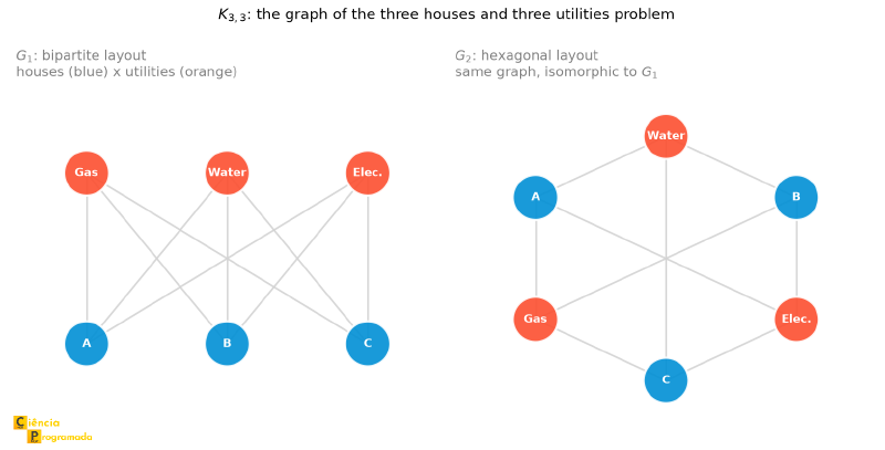
This graph is a complete bipartite graph: each house is connected to all 3 utilities, and vice versa. It is denoted \(K_{3,3}\).
Mathematically, the three houses and three utilities problem is then equivalent to asking: can we draw the graph \(K_{3,3}\) so that no edge crosses another? In other words, is the complete bipartite graph \(K_{3,3}\) planar? The answer, which we will prove later, is no.
Planar Graphs #
A graph \(G\) is planar if it can be drawn in the plane so that no pair of edges crosses, except at vertices. Such a drawing is called a plane representation (or plane embedding) of \(G\) (see the entry Planar graph).
Example 1: the complete graph \(K_4\)
Statement: The most obvious drawing of \(K_4\) (a square with both diagonals) has crossing edges. Does this mean that \(K_4\) is non-planar?
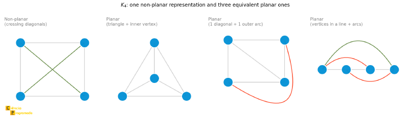
Solution: No. The figure shows this non-planar representation next to three equivalent planar representations of the same graph \(K_4\), all without crossing edges, just by rearranging the vertices. Hence \(K_4\) is planar: at least one plane representation of it exists, even if other drawings of the same graph have crossings.
Example 2: the graphs \(K_5\) and \(K_{3,3}\)
Statement: Is it possible to draw a plane representation of the graphs \(K_5\) (the complete graph on 5 vertices) and \(K_{3,3}\) (the graph of the utilities problem, from the previous section)?
Solution: No. However you reposition the vertices, at least one crossing always remains; the following figure shows both graphs drawn this way:
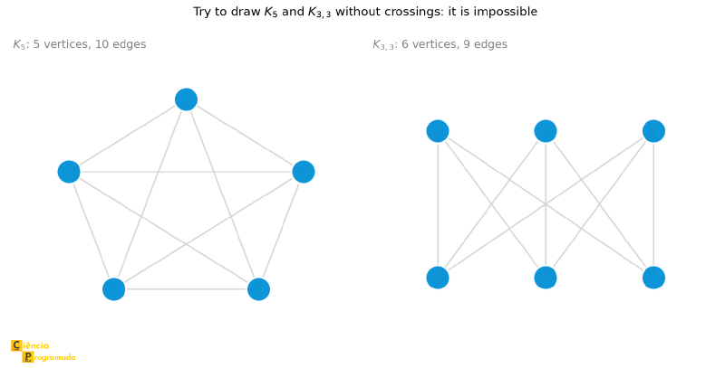
We will rigorously prove later, using Euler’s Formula, that neither of them admits a plane representation.
Other immediate examples:
- Trees: always planar, since they can be drawn without crossings starting from a root, level by level, with the children of each vertex side by side right below it
- \(C_n\) (cycles): planar for every \(n\)
Faces of a Planar Graph #
When we draw a planar graph in the plane, the edges divide the plane into regions called faces.
If \(G\) is a planar graph, every plane representation of \(G\) divides the plane into regions called faces. One of these regions is unbounded and is called the outer face.
An important property: if \(G\) is a planar graph, every plane representation of \(G\) has the same number of faces, denoted \(f\). In other words, although the drawing of a planar graph is not unique, the number of faces is an invariant of the graph: no matter how you draw it, the number of regions created is always the same.
Example: three representations of \(K_4\), always with 4 faces
Statement: Consider \(K_4\) (\(n = 4\) vertices, \(m = 6\) edges) and three different plane representations: \(R_1\), an outer triangle with an inner vertex connected to the three corners; \(R_2\), a square with a diagonal and an outer arc; \(R_3\), four vertices in a line with arc edges above and below. Do all three have the same number of faces?
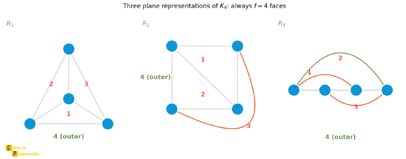
Solution: Yes. Although they are completely different drawings of the same graph, the three representations have exactly \(f = 4\) faces; in \(R_1\), for example, there are 3 inner (triangular) faces plus 1 outer face. This coincidence is no accident: it is exactly what Euler’s Formula, below, formalizes.
Euler’s Formula #
If \(G\) is a connected planar graph with \(n\) vertices, \(m\) edges, and \(f\) faces, then:
$$n - m + f = 2$$Proof:
Consider a spanning tree \(T\) of \(G\) (removing \(m - (n-1)\) edges):
- \(T\) has \(n\) vertices, \(n-1\) edges, 1 face (the whole plane): \(n - (n-1) + 1 = 2\). ✓
Now, we add an edge back to the graph. Each added edge connects two vertices that are already in the drawing and creates exactly one new face (it splits an existing face in two):
- \(\Delta n = 0\), \(\Delta m = +1\), \(\Delta f = +1\)
- The equation \(n - m + f = 2\) still holds
Adding all the remaining \(m - (n-1)\) edges, we arrive at \(G\) with the equality preserved. Therefore, \(n - m + f = 2\) for every connected planar graph, which is what we wanted to prove. \(\blacksquare\)
The formula is the planar case of a more general invariant of topology, the Euler characteristic.
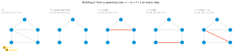
Example: building the graph from the spanning tree
Statement: What does the construction used in the proof above look like, step by step: start from a spanning tree \(T_G\) of a graph \(G\) and put the missing edges back, one by one?
Solution: The following figure illustrates the sequence: \(T_G\) has only 1 face, the whole plane. Each edge put back connects two vertices that already exist in the drawing and cuts an existing face in two: that is why \(n\) stays fixed while \(m\) and \(f\) increase together, always by 1, preserving \(n - m + f = 2\) at every step.
Check with \(K_4\)
\(n = 4\), \(m = 6\): \(4 - 6 + f = 2 \implies f = 4\). Confirmed! ✓
If \(G\) is planar with \(c\) connected components (the \(\omega(G)\) from the article on paths), the formula becomes \(n - m + f = 1 + c\). Applying Euler’s Formula to each component and adding up, we get \(n - m + (\text{sum of the faces}) = 2c\); but the outer face was counted \(c\) times, once per component, and it is only one. Removing the \(c - 1\) repetitions, \(n - m + f = 2c - (c - 1) = 1 + c\). With \(c = 1\), we are back to \(n - m + f = 2\).
Corollaries: Bounds for Planar Graphs #
Euler’s Formula implies important inequalities that bound the number of edges in planar graphs.
Corollary 1: General Bound #
If \(G\) is connected, planar, and \(n \geq 3\), then:
$$m \leq 3n - 6$$Proof: Each face is bounded by at least 3 edges. Each edge bounds at most 2 faces. Hence:
$$3f \leq 2m \implies f \leq \frac{2m}{3}$$From Euler’s Formula: \(f = 2 - n + m\). Substituting:
$$3(2 - n + m) \leq 2m \implies 6 - 3n + 3m \leq 2m \implies m \leq 3n - 6$$Therefore, every connected planar graph with \(n \geq 3\) vertices has \(m \leq 3n - 6\), which is what we wanted to prove. \(\blacksquare\)
Corollary 2: Triangle-Free Graphs #
If \(G\) is connected, planar, \(n \geq 3\), and triangle-free (no cycles of length 3), then:
$$m \leq 2n - 4$$Proof: Without triangles, each face is bounded by at least 4 edges. Hence:
$$4f \leq 2m \implies 4(2-n+m) \leq 2m \implies m \leq 2n - 4$$Therefore, every connected planar triangle-free graph with \(n \geq 3\) vertices has \(m \leq 2n - 4\), which is what we wanted to prove. \(\blacksquare\)
Corollary 3: \(K_5\) Is Not Planar #
\(K_5\) has \(n = 5\), \(m = 10\). If it were planar: \(m \leq 3(5) - 6 = 9\). But \(10 > 9\). Contradiction. Therefore, \(K_5\) is not planar, which is what we wanted to prove. \(\blacksquare\)
Corollary 4: \(K_{3,3}\) Is Not Planar #
\(K_{3,3}\) has \(n = 6\) vertices, \(m = 9\) edges, and is bipartite: it contains no triangles.
Suppose \(K_{3,3}\) is planar and let us try applying Corollary 1 first: the relation requires \(m \leq 3n - 6\). But \(m = 9 < 3(6) - 6 = 12\), so the inequality is satisfied and Corollary 1 alone does not let us conclude anything about the planarity of \(K_{3,3}\).
Since \(K_{3,3}\) has no triangles, we can apply Corollary 2, which is more restrictive: the relation requires \(m \leq 2n - 4\). But \(m = 9 > 2(6) - 4 = 8\). Contradiction.
Therefore, \(K_{3,3}\) is not planar, which is what we wanted to prove. \(\blacksquare\)
The inequalities \(m \leq 3n - 6\) and \(m \leq 2n - 4\) are necessary for planarity, but not sufficient. There are graphs that satisfy these restrictions and still are not planar: that is precisely what happened above with \(K_{3,3}\) and Corollary 1.
Graphs That Contain \(K_5\) or \(K_{3,3}\) as a Subgraph #
Two simple but useful observations follow from everything we have seen so far.
Observation 1: \(K_5\) and \(K_{3,3}\) are, respectively, the non-planar graphs with the fewest possible vertices and the fewest possible edges: proven minima, not just the smallest known. As we will see with Kuratowski’s Theorem, every non-planar graph contains a subdivision of one of the two and, therefore, has at least 5 vertices and at least 9 edges.
Observation 2: If \(G\) is a planar graph, then every subgraph of \(G\) is also planar: removing vertices or edges from a drawing without crossings cannot create a crossing. Equivalently:
If a graph \(G\) contains a non-planar graph as a subgraph, then \(G\) is non-planar.
This observation is already enough to detect non-planarity in graphs much larger than \(K_5\) or \(K_{3,3}\): we just need to find one of these two structures “hidden” inside a larger graph.
Example: two non-planar graphs because they contain \(K_5\) and \(K_{3,3}\)
Statement: Consider two graphs \(G_1\) and \(G_2\):
- \(G_1\) is formed by a copy of \(K_5\) (highlighted) with an extra vertex and an extra edge hanging from one of the vertices.
- \(G_2\) is formed by a copy of \(K_{3,3}\) (highlighted) with two extra vertices hanging.
Are \(G_1\) and \(G_2\) planar?
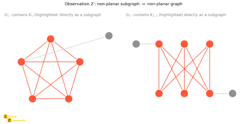
Solution: No, neither of them. Since \(G_1\) contains \(K_5\) as a subgraph, \(G_1\) is not planar. Since \(G_2\) contains \(K_{3,3}\) as a subgraph, \(G_2\) is not planar. Note that, in this example, the forbidden graph appears directly as a subgraph, without any subdivision. The next section generalizes this idea to the case where the forbidden graph appears “disguised” by subdivisions.
Graph Subdivision #
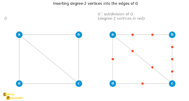
A subdivision of \(G\) is obtained by inserting degree-2 vertices into the edges of \(G\), so each edge may be replaced by a path of arbitrary length.
Intuitively, subdividing an edge means placing one or more intermediate “waypoints” on it, without changing the connection structure of the graph. The following figure shows a graph \(G\) and a subdivision \(G^{\prime}\) of it, with degree-2 vertices (in red) inserted in varying numbers on each edge.
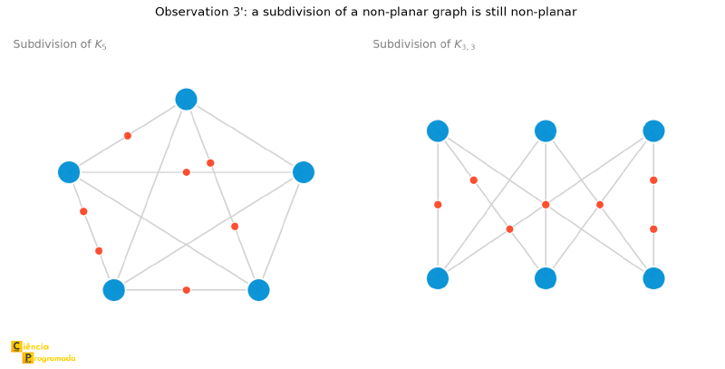
Observation 3: If \(G\) is planar, then any subdivision of \(G\) is also planar: inserting a vertex in the middle of an edge cannot create a crossing. Equivalently:
If \(G\) is a subdivision of a non-planar graph, then \(G\) is non-planar.
The following figure illustrates this observation with subdivisions of \(K_5\) and \(K_{3,3}\), with the inserted degree-2 vertices highlighted in red:
Combining Observation 2’ (subgraph, from the previous section) with Observation 3’ (subdivision), we obtain the more general result:
Observation 4: If \(G\) is a graph that contains a subdivision of \(K_5\) or of \(K_{3,3}\) as a subgraph, then \(G\) is non-planar.
Kuratowski’s Theorem #
The deepest result about planar graphs provides a complete characterization:
A graph \(G\) is planar if and only if it contains no subdivision of \(K_5\) or of \(K_{3,3}\) as a subgraph (see the entry Kuratowski’s theorem).
The direction “if \(G\) contains a subdivision of \(K_5\) or \(K_{3,3}\), then \(G\) is not planar” is already proven: it is exactly Observation 4 from the previous section. The hard and surprising part of the theorem is the converse: every graph that contains no such subdivisions is necessarily planar. That direction requires a long and technical proof, which is beyond the scope of this article.
This theorem says that \(K_5\) and \(K_{3,3}\) are, in a sense, the only obstacles to planarity. Every non-planar graph contains one of these two graphs “hidden” (possibly with subdivisions).
Although the theorem provides the complete theoretical characterization,
checking computationally whether a graph is planar led to the development of
sophisticated algorithms. The first linear-time algorithm, \(O(n)\), was
published by John Hopcroft and Robert Tarjan in 1974; in 2004, John Boyer and
Wendy Myrvold arrived at a simpler linear algorithm, which also builds the
plane drawing (see the entry
Planarity testing). In
networkx, a linear test is ready-made as nx.check_planarity.
Coloring Planar Graphs #
In the first article of the series, the Four Color Theorem appeared as a statement about maps. With the language of this article, it becomes a theorem about planar graphs, and Euler’s Formula is enough to prove a weaker version of it.
A coloring of a graph \(G\) with \(k\) colors assigns to each vertex one of \(k\) colors, so that adjacent vertices get different colors. The chromatic number \(\chi(G)\) is the smallest \(k\) for which a coloring of \(G\) with \(k\) colors exists.
Some immediate consequences of the definition:
- Vertices of the same color cannot be neighbors: they form an independent set. Coloring \(G\) with \(k\) colors is partitioning \(V(G)\) into \(k\) independent sets.
- If \(G\) contains a clique with \(k\) vertices, then \(\chi(G) \geq k\), because the vertices of the clique need all-different colors. In particular, \(\chi(K_n) = n\).
- A graph with at least one edge has \(\chi(G) = 2\) exactly when it is bipartite: the two colors are the two sides of the bipartition. That is why an odd cycle needs 3 colors.
From maps to planar graphs. Each region of a map becomes a vertex, and two regions with a common border of positive length become adjacent vertices. The resulting graph is planar: just put each vertex inside its region and connect two neighboring regions by a line that crosses the common border. Coloring the map is coloring this graph, and the theorem takes its graph theory form:
Every planar graph \(G\) has \(\chi(G) \leq 4\).
In 1879, Alfred Kempe published a proof that was accepted for more than ten years, until Percy Heawood found an error in it, in 1890, and, in the same paper, proved that five colors always suffice. The proof by Kenneth Appel and Wolfgang Haken, from 1976, reduced the problem to a huge set of configurations checked by computer. In 1996, Neil Robertson, Daniel Sanders, Paul Seymour, and Robin Thomas presented a simpler proof, still with a computer, with 633 configurations; and in 2005 Georges Gonthier and Benjamin Werner formalized a complete proof in the Coq proof assistant (see the entry Four color theorem).
Four colors without four mutually neighboring regions. The wheel with 5 spokes (a cycle \(C_5\) plus a central vertex connected to all five) is planar and does not contain \(K_4\): a copy of \(K_4\) would need three mutually adjacent vertices of the cycle, and \(C_5\) has no triangles. Even so, \(\chi = 4\). The cycle \(C_5\) is odd and needs 3 colors, and the central vertex, a neighbor of all the vertices of the cycle, cannot repeat any of them. It is the graph version of the example that the first article used to show that “not having \(K_5\)” does not, by itself, explain why four colors suffice: needing \(k\) colors does not require containing \(K_k\). The figure below shows the map and the wheel side by side, with a 4-coloring:
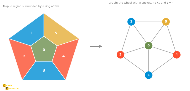
The proof of the Four Color Theorem is beyond the reach of an article, but the six-color version follows from Corollary 1 in a few lines. The starting point is a lemma.
Every planar graph has a vertex of degree at most 5.
Proof: Let \(H\) be a connected component of the planar graph \(G\); \(H\) is also planar. If \(H\) has at most 2 vertices, its vertices have degree at most 1. Otherwise, \(H\) is connected, planar, and has \(n_H \geq 3\) vertices, and Corollary 1 gives \(m_H \leq 3n_H - 6\). If every vertex of \(H\) had degree at least 6, the Handshaking Theorem would give \(2m_H = \sum d(v) \geq 6n_H\), that is, \(m_H \geq 3n_H > 3n_H - 6\), a contradiction. Therefore, \(H\), and with it \(G\), has a vertex of degree at most 5, which is what we wanted to prove. \(\blacksquare\)
Every planar graph \(G\) has \(\chi(G) \leq 6\).
Proof by induction on the number \(n\) of vertices:
Base case: if \(n \leq 6\), just give a different color to each vertex.
Inductive hypothesis: suppose every planar graph with \(n - 1\) vertices (\(n \geq 7\)) can be colored with 6 colors.
Inductive step: let \(G\) be planar with \(n\) vertices. By the lemma, \(G\) has a vertex \(v\) with \(d(v) \leq 5\). Removing \(v\) and its edges, we get \(G - v\), which is planar (it is a subgraph of \(G\), Observation 2) and has \(n - 1\) vertices; by the inductive hypothesis, \(G - v\) can be colored with 6 colors. The at most 5 neighbors of \(v\) use at most 5 of these colors, and at least one is left for \(v\).
Therefore, every planar graph with \(n\) vertices can be colored with 6 colors, that is, \(\chi(G) \leq 6\), which is what we wanted to prove. \(\blacksquare\)
With more work (swapping colors along paths of two alternating colors, the “Kempe chains”), the same lemma gives Heawood’s Five Color Theorem. To get to four, nobody has found an argument of that size.
Checking with code
networkx tests planarity with nx.check_planarity and colors with
nx.greedy_color, which goes through the vertices in some order and gives
each one the smallest color not yet used by its neighbors. Greedy coloring
does not guarantee the minimum, but with the "smallest_last" strategy it
repeats the Six Color proof: it removes a vertex of minimum degree, then
another, and colors in the reverse order. That is why, on a planar graph,
this strategy never uses more than 6 colors.
import networkx as nx

wheel = nx.wheel_graph(6)  # vertex 0 in the center, connected to the cycle 1-2-3-4-5
print(nx.check_planarity(wheel)[0])  # True
colors = nx.greedy_color(wheel, strategy="largest_first")
print(colors)  # {0: 0, 1: 1, 2: 2, 3: 1, 4: 2, 5: 3}
print(len(set(colors.values())))  # 4

icosahedron = nx.icosahedral_graph()  # planar, all vertices with degree 5
print(nx.check_planarity(icosahedron)[0])  # True
colors = nx.greedy_color(icosahedron, strategy="smallest_last")
print(len(set(colors.values())))  # 4
The wheel uses exactly the four colors it needs. The icosahedron shows that the lemma cannot be improved (every vertex there has degree 5), and even so greedy coloring finds 4 colors.
Application: conflict-free schedules
Five committees in a company need to meet, and two committees with a member in common cannot meet at the same time. In the conflict graph, each committee is a vertex and each shared member becomes an edge; the time slots are the colors, and the minimum number of time slots is \(\chi(G)\). The same modeling distributes radio frequencies among neighboring antennas and processor registers among the variables of a program.
import networkx as nx

conflicts = nx.Graph([
    ("Budget", "Personnel"), ("Budget", "Construction"),
    ("Personnel", "Construction"), ("Personnel", "Technology"),
    ("Construction", "Technology"), ("Technology", "Events"),
])
schedules = nx.greedy_color(conflicts, strategy="largest_first")
print(schedules)
# Output: {'Personnel': 0, 'Construction': 1, 'Technology': 2, 'Budget': 2, 'Events': 0}
print(max(schedules.values()) + 1)  # 3 time slots
Three time slots are the minimum: Budget, Personnel, and Construction form a clique with three vertices, and a clique with \(k\) vertices requires \(k\) colors.
Summary Table #
| Concept | Expression/Definition |
|---|---|
| Planar graph | Drawable in the plane without crossing edges |
| Face invariance | Every plane representation of a connected graph has the same number of faces \(f\) |
| Euler’s Formula | \(n - m + f = 2\) (connected planar graph) |
| General bound | \(m \leq 3n - 6\) (necessary; \(n \geq 3\)) |
| Triangle-free | \(m \leq 2n - 4\) (necessary; \(n \geq 3\)) |
| \(K_5\) | \(m = 10 > 9 = 3(5)-6\) → non-planar |
| \(K_{3,3}\) | \(m = 9 > 8 = 2(6)-4\) → non-planar |
| Planarity inheritance | A subgraph of a planar graph is planar → a graph with a non-planar subgraph is non-planar |
| Kuratowski | Planar \(\iff\) no subdivision of \(K_5\) or \(K_{3,3}\) as a subgraph |
| General Euler’s Formula | \(n - m + f = 1 + c\) (planar graph with \(c\) components) |
| Chromatic number | \(\chi(G)\) = smallest number of colors with neighbors of different colors |
| Minimum degree in planar graphs | Every planar graph has a vertex of degree \(\leq 5\) |
| Six Color Theorem | Planar graph \(\Rightarrow \chi(G) \leq 6\) (proof by induction) |
| Four Color Theorem | Planar graph \(\Rightarrow \chi(G) \leq 4\) (Appel and Haken, 1976) |
Exercises #
Exercise 1: Number of faces
A connected planar graph has 8 vertices and 12 edges. How many faces does it have?
Solution
From Euler’s Formula: \(f = 2 - n + m = 2 - 8 + 12 = 6\) faces.
Exercise 2: Is \(K_{2,4}\) planar?
Statement: Is the complete bipartite graph \(K_{2,4}\) planar?
Solution
\(K_{2,4}\) has \(n = 6\), \(m = 8\). It is bipartite (triangle-free). By Corollary 2: \(m \leq 2(6) - 4 = 8\). Since \(8 \leq 8\), the corollary does not rule out planarity. In fact, \(K_{2,4}\) is planar: it is possible to draw it without crossings.
Exercise 3: non-planar subgraph
A graph \(G\) has 8 vertices and 14 edges, and you discover that 5 of those vertices, together with 10 of the edges among them, form a copy of \(K_5\). What can be concluded about the planarity of \(G\)?
Solution
By Observation 2’, if \(G\) contains a non-planar graph (\(K_5\)) as a subgraph, then \(G\) is non-planar, regardless of what happens in the other 3 vertices and the other 4 edges.
Next Steps #
Everything in this article dealt with drawability: whether a graph can be placed in the plane without crossing edges. At no point did we ask whether the connections have a single direction: whether going from \(A\) to \(B\) is the same as going from \(B\) to \(A\). That is exactly the limitation that closes this stage of the series: planarity says nothing about the direction of the connections. In the next article of this series, we study directed graphs: when the direction of the connections matters.


