

If you have ever used a file system, a binary search data structure, a heap, or parsed the syntax of a program, you have already worked with trees. They are among the most widely used data structures in computer science.
Within graph theory, trees also hold a special place: they are the simplest family of graphs and the one with the friendliest properties. That is why, whenever we want to prove a general result about graphs, the most natural strategy is to check first whether it holds for trees. If it fails even in this simplest case, there is no hope for the general case; if it holds, a good part of the proof work is already done. Trees also show up outside computing, describing everything from the structure of molecules in chemistry to syntactic analysis in linguistics, but it is in computing that they are most useful.
Why Do Trees Matter? #
Trees are, at the same time, the simplest theoretical model in graph theory and one of the most widely used data structures in practice:
- File systems: folders and files naturally form a rooted tree, where each folder is the child of exactly one parent folder.
- Compilers and interpreters: parsing a program produces an abstract syntax tree (AST), used to generate code or to interpret the language.
- Efficient search structures: binary search trees and heaps organize data hierarchically to make search, insertion, and removal fast, as long as the tree stays balanced, with small height.
- Minimum-cost networks: finding the minimum spanning tree of a network (the cheapest way to keep everything connected, with no redundant cycles) is a classic optimization problem in telecommunications and logistics.
Definition of a Tree #
A tree is a connected and acyclic (cycle-free) graph.
An acyclic graph is a forest: each connected component of a forest is a tree.
The definition of a tree is minimalist: a tree has the minimum number of edges needed to keep it connected, and removing any edge disconnects it.
The following three trees illustrate this definition well:
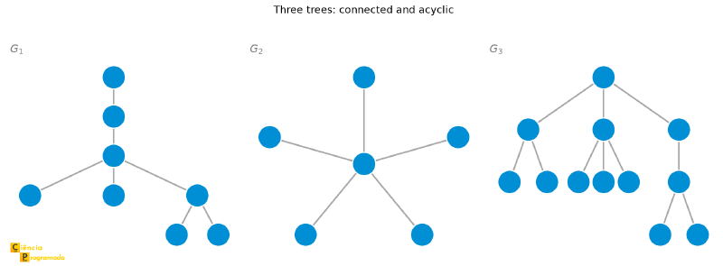
The example above shows three trees that are quite different from one another (one looks like a crooked path, another is a star, the third branches into several levels), but all of them share the two properties that define the category: they are connected and have no cycles.
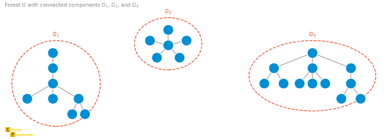
A forest, in turn, is what is left when we give up connectivity but keep the absence of cycles: each isolated piece (each connected component) is, by itself, a tree. The same three trees above, for example, can be seen as the three connected components of a single forest:
Leaves #
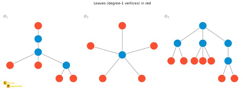
A leaf (or pendant vertex) is a vertex \(v\) such that \(d(v) = 1\).
In the same three trees, the leaves (highlighted in red) are exactly the vertices of degree 1, at the tips of the branches:
A Characterization of Trees #
The following result connects the definition of a tree (connected and acyclic) to an equivalent property, but one stated in a different way, in terms of paths:
A graph \(G\) is a tree if and only if there is a unique path between every pair of vertices of \(G\).
Proof:
(⇒) Let \(G\) be a tree. By definition \(G\) is connected, so between each pair of vertices \(v\) and \(w\) there is at least one path. It remains to show that this path is unique.
Suppose, for contradiction, that there are two distinct paths \(P_1\) and \(P_2\) between \(v\) and \(w\). Since the paths are distinct but share the endpoints \(v\) and \(w\), there are necessarily two vertices \(t_1\) and \(t_2\) (possibly \(t_1 = v\) and \(t_2 = w\), if the paths touch only at the endpoints) such that, between \(t_1\) and \(t_2\), the subpaths of \(P_1\) and \(P_2\) are vertex-disjoint, that is, \(t_1\) and \(t_2\) are the first point where the paths separate and the next point where they meet again.
The subpath of \(P_1\) between \(t_1\) and \(t_2\), joined to the subpath of \(P_2\) between \(t_1\) and \(t_2\) (traversed in the opposite direction), forms a cycle. This contradicts the fact that \(G\) is acyclic. Hence the path between \(v\) and \(w\) is unique.
(⇐) Suppose there is a unique path between each pair of vertices of \(G\). In particular, there is at least one path between each pair of vertices, so \(G\) is connected.
It remains to show that \(G\) is acyclic. Suppose, for contradiction, that \(C\) is a cycle of \(G\), and let \((v, w)\) be an edge of \(C\). Then there are two distinct paths between \(v\) and \(w\): the edge \((v,w)\) itself and the path \(C - (v,w)\) (the rest of the cycle). This contradicts the unique-path hypothesis. Hence \(G\) is acyclic.
Since \(G\) is connected and acyclic, \(G\) is a tree. Therefore, a graph is a tree if and only if there is a unique path between each pair of its vertices, which is what we wanted to prove. \(\blacksquare\)
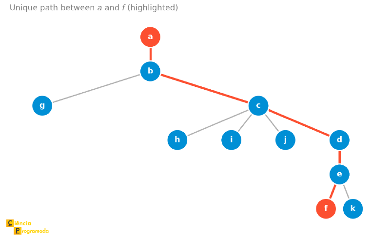
In the tree below, for example, there is a unique path between vertices \(a\) and \(f\), highlighted in red:
Trees and the Number of Edges #
If \(G\) is a tree with \(n\) vertices, then \(G\) has exactly \(n - 1\) edges.
Proof by strong induction on \(n\):
Base case: \(n = 1\). A tree with 1 vertex (the trivial graph) has 0 edges. \(n - 1 = 0\). ✓
Inductive hypothesis: suppose the result holds for every tree with fewer than \(n\) vertices (\(n \geq 1\)).
Inductive step: let \(T\) be a tree with \(n\) vertices (\(n > 1\)). Since \(n > 1\), \(T\) contains at least one edge \(e = (v, w)\). Let \(T^{\prime}\) be the graph obtained by removing \(e\) from \(T\) (without removing the vertices).
By Theorem 1, the unique path between \(v\) and \(w\) in \(T\) is the edge \(e\) itself. When \(e\) is removed, \(v\) and \(w\) are no longer connected in \(T^{\prime}\): they end up in two distinct connected components of \(T^{\prime}\). And there are no other components: every vertex \(x\) remains linked to \(v\) or to \(w\), because the path from \(x\) to \(v\) in \(T\), if it uses the edge \(e\), passes through \(w\) right before it. Let \(T_1\) and \(T_2\) be these two components. Each of them is acyclic (since it is a subgraph of a tree) and connected (it is a connected component); hence \(T_1\) and \(T_2\) are trees, each with fewer than \(n\) vertices.
By the inductive hypothesis, applied to \(T_1\) and \(T_2\):
$$|E(T_1)| = |V(T_1)| - 1 \qquad \text{and} \qquad |E(T_2)| = |V(T_2)| - 1$$Since \(V(T_1) \cup V(T_2) = V(T)\) and \(E(T_1) \cup E(T_2) \cup \{e\} = E(T)\), we have:
$$n = |V(T)| = |V(T_1)| + |V(T_2)|$$$$m = |E(T)| = |E(T_1)| + |E(T_2)| + 1 = \big(|V(T_1)| - 1\big) + \big(|V(T_2)| - 1\big) + 1 = |V(T_1)| + |V(T_2)| - 1 = n - 1$$
Therefore, by induction, every tree with \(n\) vertices has \(m = n - 1\) edges, which is what we wanted to prove. \(\blacksquare\)
Checking with code
The proof above holds for any \(n\), but there is nothing like generating random trees of very different sizes and checking the relation \(m = n-1\) on each one:
import networkx as nx

for n in [5, 10, 20, 50, 100]:
    T = nx.random_labeled_tree(n, seed=42)
    m, v = T.number_of_edges(), T.number_of_nodes()
    print(f"n={v:>3}: |V|={v:>3}, |E|={m:>3}, |E| == |V|-1? {m == v - 1}")
n= 5: |V|= 5, |E|= 4, |E| == |V|-1? True
n= 10: |V|= 10, |E|= 9, |E| == |V|-1? True
n= 20: |V|= 20, |E|= 19, |E| == |V|-1? True
n= 50: |V|= 50, |E|= 49, |E| == |V|-1? True
n=100: |V|=100, |E|= 99, |E| == |V|-1? Truenx.random_labeled_tree(n) draws a random tree from among all
\(n^{n-2}\) possible labeled trees with \(n\) vertices (the same
Cayley’s formula that reappears later, in the spanning tree section), and in
every one of them, without exception, the number of edges is exactly the
number of vertices minus one.
The converse is also true: a connected graph with \(n\) vertices and \(n-1\) edges is necessarily a tree. Moreover, any two of the three conditions below imply the third:
- \(G\) is connected
- \(G\) is acyclic
- \(|E| = |V| - 1\)
Center of a Tree #
Before talking about the center of a tree specifically, it is worth recalling the general definition of eccentricity and center of a graph, which we already saw when studying distance, eccentricity, and diameter.
Let \(G = (V, E)\) be a graph. The eccentricity of a vertex \(v\) is
$$e(v) = \max_{w \in V} d(v, w)$$that is, the greatest distance from \(v\) to any other vertex of the graph. The center of \(G\) is the set
$$c(G) = \{w \in V \mid e(w) \text{ is minimum}\}$$In any graph, \(1 \leq |c(G)| \leq |V(G)|\).
In an arbitrary graph, the center can have any size between 1 and all the vertices. In trees, however, this number is always very small:
The center of any tree consists of a single vertex or of two adjacent vertices.
Proof: the argument rests on three facts.
Fact 1: in a tree with at least three vertices, no leaf belongs to the center. If \(f\) is a leaf and \(u\) is its only neighbor, every path leaving \(f\) goes through \(u\); hence \(d(f, w) = 1 + d(u, w)\) for every \(w \neq f\), and \(e(f) = e(u) + 1\). The leaf is always one unit farther from everything than its neighbor.
Fact 2: if we remove all the leaves of a tree \(G\) (and the edges incident to them), obtaining a graph \(G^{\prime}\), every vertex of \(G^{\prime}\) has eccentricity exactly one unit smaller in \(G^{\prime}\) than it had in \(G\). This happens because, in a tree, the longest paths from any vertex necessarily end at leaves; removing the leaves shortens these paths by exactly 1.
Fact 3: \(c(G) = c(G^{\prime})\). Since all vertices of \(G^{\prime}\) had their eccentricity reduced by the same amount (Fact 2), and the removed leaves were not in the center (Fact 1), the set of vertices of minimum eccentricity does not change.
Facts 1, 2, and 3 justify the following iterative algorithm for finding the center:
-
1
Remove the leaves
Remove all the leaves of \(G\) (along with the incident edges). -
2
Repeat
Repeat the procedure on the remaining graph. -
3
Stop at one or two vertices
Stop when a single vertex remains, or two vertices joined by an edge: that is the center.
Since the graph has a finite number of vertices and each round removes at least one leaf, the process terminates, and it can only stop at a single vertex or at two vertices joined by an edge (if three or more vertices were left, at least two of them would still be leaves, and the next round would remove them). Therefore, the center of any tree is a single vertex or two adjacent vertices, which is what we wanted to prove. \(\blacksquare\)
Balanced trees #
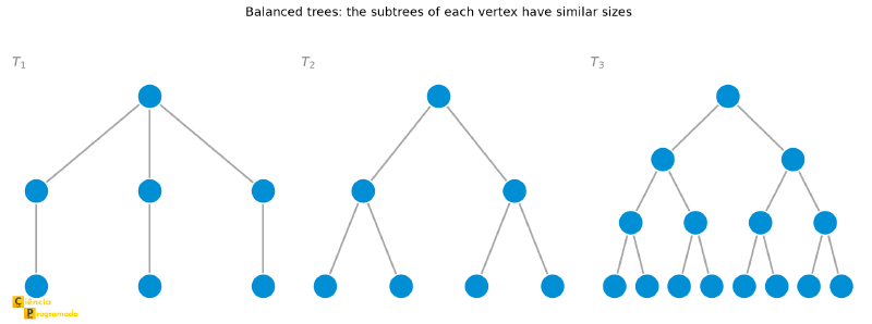
A neighboring concept, widely used in data structures, is that of a balanced tree: a rooted tree in which the subtrees hanging from each vertex have similar sizes, so that no branch is much longer than the others. The exact criterion changes from one structure to another. In AVL trees (named after the initials of Georgy Adelson-Velsky and Evgenii Landis, who published them in 1962), the heights of the two subtrees of any vertex differ by at most 1; in red-black trees, a rule about vertex colors guarantees that no path from the root to a leaf is more than twice as long as another. In both cases, the tree rebalances itself at each insertion or removal, which keeps the height logarithmic in the number of elements, and it is precisely this small height that makes searches, insertions, and removals fast in these structures.
The figure below shows three balanced trees:
Why balancing matters: balanced vs. degenerate height
“Logarithmic height” is an abstract phrase until you see how big the difference is in practice. Let us compare the height of a balanced binary tree (generated with all levels complete) with that of a degenerate tree, a chain of only-children, like a linked list, which is what you get, for example, by inserting already sorted data into a plain binary search tree, without rebalancing:
import networkx as nx
import math

for h in [1, 2, 3, 4, 10]:
    balanced_tree = nx.balanced_tree(r=2, h=h)
    n = balanced_tree.number_of_nodes()
    balanced_height = nx.eccentricity(balanced_tree, v=0)  # 0 is the root
    degenerate_height = n - 1  # chain with n vertices, rooted at one end
    print(f"n={n:>5} | balanced height={balanced_height:>2} | degenerate height={degenerate_height:>5}")
n= 3 | balanced height= 1 | degenerate height= 2
n= 7 | balanced height= 2 | degenerate height= 6
n= 15 | balanced height= 3 | degenerate height= 14
n= 31 | balanced height= 4 | degenerate height= 30
n= 2047 | balanced height=10 | degenerate height= 2046With only 2,047 elements, the balanced tree has height 10, that is, any search finds what it is looking for in at most 10 steps, while the degenerate version has height 2,046, practically going through all the elements one by one (the same cost as searching a list). It is exactly this difference, which only grows as \(n\) increases, that makes balanced trees indispensable in high-performance search structures.
Examples #
Example 1: center of a cross-shaped graph
Statement: Find the center of the cross-shaped tree below, with a central vertex \(c\) and four “arms” of lengths 1, 2, 2, and 4 extending from it.
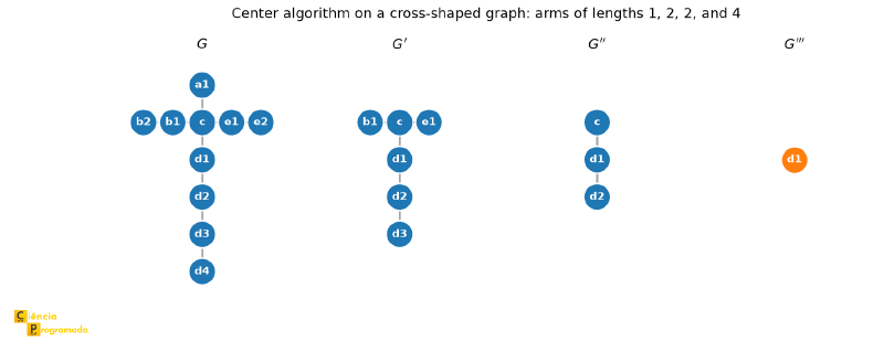
Solution: Applying the algorithm: in each round, we remove the current leaves (the tips of each arm). Since the arms have different lengths, some disappear before others, and the process converges to a single vertex. Note that this vertex is not the central hub \(c\) from which the arms extend: it is a vertex in the middle of the longest arm. The center of a tree is defined by minimum eccentricity, not by the “visually most central” position in the drawing, and that is why the algorithm, and not intuition, is the reliable tool.
Example 2: center of a branched tree
Statement: Find the center of the branched tree below (it is neither a simple path nor a cross).
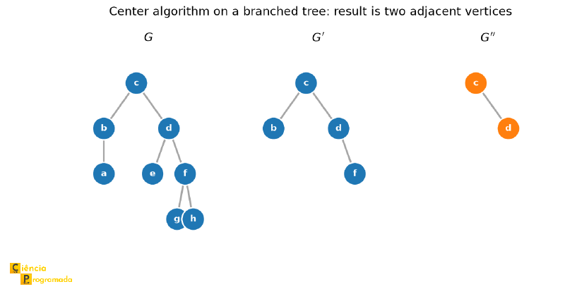
Solution: Applying the same leaf-removal algorithm, the procedure ends with two adjacent vertices. Note that, even in a tree with a much more irregular structure than a path or a cross, the algorithm keeps working in exactly the same way, and the result is still 1 or 2 adjacent vertices, as the theorem guarantees.
Checking with code
Implementing the leaf-removal algorithm by hand is a good exercise, but
networkx already ships this computation as nx.center. Let us apply it to
the two graphs we have just solved by hand:
import networkx as nx

G_cross = nx.Graph()
G_cross.add_edges_from([
    ("c", "a1"),
    ("c", "b1"), ("b1", "b2"),
    ("c", "e1"), ("e1", "e2"),
    ("c", "d1"), ("d1", "d2"), ("d2", "d3"), ("d3", "d4"),
])
print("Center of the cross graph:", sorted(nx.center(G_cross)))

G_branched = nx.Graph()
G_branched.add_edges_from([
    ("c", "b"), ("c", "d"),
    ("b", "a"),
    ("d", "e"), ("d", "f"),
    ("f", "g"), ("f", "h"),
])
print("Center of the branched tree:", sorted(nx.center(G_branched)))
Center of the cross graph: ['d1']
Center of the branched tree: ['c', 'd']Both results match exactly what we found by hand by removing leaves round by round, including the “surprise” of the first example, in which the center is not the vertex \(c\) from which the arms extend, but \(d_1\), in the middle of the longest arm.
Spanning Tree #
A spanning tree of a connected graph \(G\) is a spanning subgraph of \(G\) that is a tree, that is, a subgraph with all \(n\) vertices of \(G\) and \(n-1\) edges forming a tree.
Every spanning tree is obtained from \(G\) by removing exactly \(|E| - (n-1)\) edges without disconnecting the graph.
For every connected graph \(G\), it is always possible to find a spanning tree systematically: select edges of \(G\), one at a time, so that no cycle is created, and repeat this procedure until \(n-1\) edges have been chosen (or, which amounts to the same thing in a connected graph, until no remaining edge can be added without closing a cycle). It is not enough to stop when all vertices appear in some chosen edge: in the path \(a - b - c - d\), the edges \((a,b)\) and \((c,d)\) already touch all four vertices, but they form a forest, not a tree.
Choosing edges without closing cycles is the most basic principle behind building a spanning tree, and it is from this principle that the best-known algorithms are built:
- Prim’s algorithm and Kruskal’s algorithm: they apply this same idea of selecting edges without creating cycles, but always choosing the available edge of least weight, to find the minimum spanning tree (the one of least total cost) in weighted graphs
- BFS (breadth-first search) and DFS (depth-first search): they naturally produce a spanning tree as they traverse the graph, marking as a tree edge each edge used to reach a vertex not yet visited
Checking with code
Let us see breadth-first search producing a spanning tree in practice, using the same graph \(G\) as the examples that follow (vertices \(a,b,c,d,e,f\), with \(a\) adjacent to \(b\), \(c\), \(e\), and \(f\)):
import networkx as nx

G = nx.Graph()
G.add_edges_from([
    ("a", "b"), ("a", "c"), ("b", "c"),
    ("c", "e"), ("a", "e"),
    ("e", "f"), ("a", "f"),
    ("e", "d"), ("c", "d"),
])

T_bfs = nx.bfs_tree(G, "a")
print("Edges of the BFS tree from a:", sorted(tuple(sorted(e)) for e in T_bfs.edges()))
print("Is it a tree?", nx.is_tree(T_bfs.to_undirected()))
Edges of the BFS tree from a: [('a', 'b'), ('a', 'c'), ('a', 'e'), ('a', 'f'), ('c', 'd')]
Is it a tree? TrueBreadth-first search from \(a\) first visits all the direct neighbors of \(a\) (\(b\), \(c\), \(e\), \(f\)) and only then reaches \(d\), through \(c\). The result is a third spanning tree of \(G\), different from the two we will see next in Examples 1 and 2, yet another confirmation that the method used to build the spanning tree (manual edge selection, BFS, DFS, …) determines which specific tree you get.
Example 1: two different spanning trees
Statement: Find two different spanning trees of the graph \(G\) below, with vertices \(a, b, c, d, e, f\) and containing some cycles.
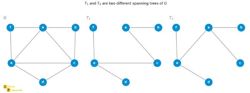
Solution: \(T_1\) and \(T_2\) are two distinct spanning trees of \(G\), both connected, acyclic, and covering all the vertices of \(G\), but using different sets of edges. This illustrates that the spanning tree of a graph is, in general, not unique.
Example 2: the order in which edges are chosen matters
Statement: Apply the edge-selection algorithm to the graph \(G\) with the edge list \(\{(a,b), (a,c), (b,c), (c,e), (a,e), (e,f), (a,f), (e,d), (c,d)\}\), going through it in that order.
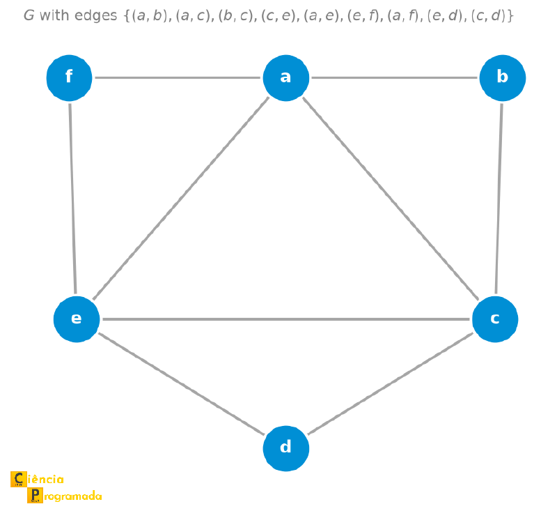
Solution: Applying the edge-selection algorithm in this order, avoiding cycles at each step, we obtain the spanning tree \(T_1\) from the previous example. If we went through the edge list in another order, we might have chosen different edges at the points where there was more than one cycle-free option, and the result would be a different, though equally valid, spanning tree (this is exactly what happens in Exercise 3 below, which produces \(T_2\)).
How many spanning trees can a graph have?
A connected graph with \(n\) vertices can have many distinct spanning trees. For the complete graph \(K_n\), Cayley’s formula shows that this number is \(n^{n-2}\), the same as the number of trees with \(n\) labeled vertices, a quantity that grows very rapidly with \(n\). The name honors Arthur Cayley, who published a note about it in 1889, but the formula had already been obtained by Carl Wilhelm Borchardt in 1860 (see the Cayley’s formula entry). This result goes beyond what we need here, but it helps explain why the choice of edge-selection criterion (such as minimum weight, in the case of Prim and Kruskal) is so important: among exponentially many possible spanning trees, we usually want one specific tree.
networkx computes this number directly (using Kirchhoff’s Matrix-Tree
Theorem, without having to enumerate the trees one by one), and the result
matches Cayley’s formula exactly:
import networkx as nx

for n in [2, 3, 4, 5, 6]:
    K_n = nx.complete_graph(n)
    count = nx.number_of_spanning_trees(K_n)
    formula = n ** (n - 2)
    print(f"n={n}: nx.number_of_spanning_trees = {count:.0f} | n**(n-2) = {formula}")
n=2: nx.number_of_spanning_trees = 1 | n**(n-2) = 1
n=3: nx.number_of_spanning_trees = 3 | n**(n-2) = 3
n=4: nx.number_of_spanning_trees = 16 | n**(n-2) = 16
n=5: nx.number_of_spanning_trees = 125 | n**(n-2) = 125
n=6: nx.number_of_spanning_trees = 1296 | n**(n-2) = 1296Rooted Trees #
In computing, we often use trees with a designated root. Given a tree \(T = (V, E)\), we just pick any vertex \(v\) and call it the root. The tree is then called a rooted tree, and its usual graphical representation (root at the top, branches going down) gains a well-defined hierarchy.
For graph theory, a tree is just a connected acyclic graph: it has no root, no order among the neighbors of a vertex, no “left” and “right”. The tree in data structures is richer: a binary search tree has a fixed root, the parent/child hierarchy, and the distinction between left child and right child. That is why two different binary trees (the root \(r\) with a single child \(x\) on the left, and the same root with \(x\) on the right) are the same graph: the vertices \(r\) and \(x\) joined by an edge.
Example: choosing a root
Statement: Consider a tree with no defined root, with vertices \(a\) through \(n\). Choose vertex \(d\) as the root and redraw the tree accordingly.
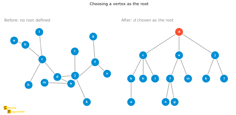
Solution: by choosing vertex \(d\) as the root, the same tree is drawn with \(d\) at the top and the other vertices arranged in levels below it.
With a root \(r\) fixed, we define:
Let \(v\) and \(w\) be two vertices of a rooted tree \(T\) with root \(r\). If \(v\) belongs to the path from \(r\) to \(w\), then \(v\) is an ancestor of \(w\), and \(w\) is a descendant of \(v\). If, in addition, \((v, w)\) is an edge, then \(v\) is the parent of \(w\) (and \(w\) is a child of \(v\)).
The root is the only vertex with no parent; the leaves are the vertices with no children.
Example: ancestor, descendant, parent, and child
Statement: In the rooted tree \(T\) below (root \(r\), children \(b\) and \(c\) of \(r\), children \(d\) and \(e\) of \(c\), and children \(f\) and \(g\) of \(e\)), identify the ancestry and kinship relations among some vertices.
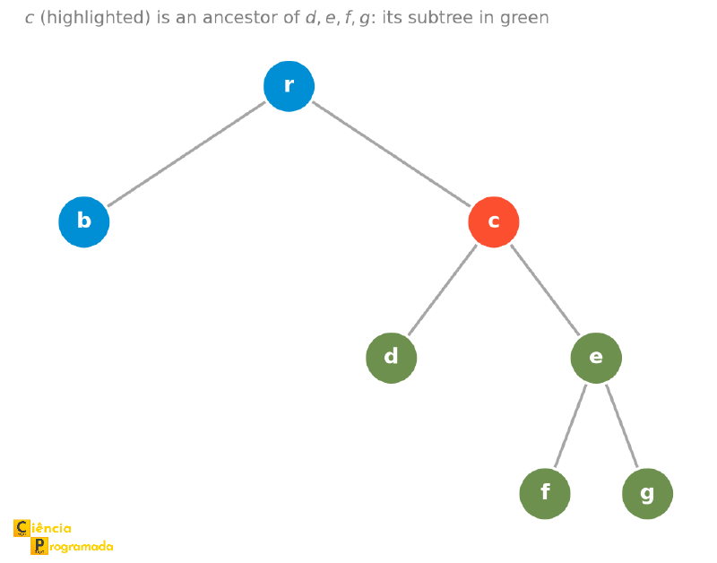
Solution:
- \(c\) is an ancestor of \(d\), \(e\), \(f\), and \(g\)
- \(c\) is the parent of \(d\) and of \(e\)
- \(b\) is neither an ancestor nor a descendant of \(c\): they are on different branches of the tree
- \(b\) and \(c\) are children of the root \(r\)
The level and the height are also defined from the root:
Let \(T\) be a rooted tree with root \(r\). The level of a vertex \(v\), denoted \(\text{level}(v)\), is the length of the unique path from \(r\) to \(v\). The height of \(T\) is the greatest level among all vertices:
$$\text{height}(T) = \max_{v \in V} \text{level}(v)$$
Example: level and height
Statement: In the same tree as the previous example (root \(r\), children \(b\) and \(c\), grandchildren \(d\) and \(e\), great-grandchildren \(f\) and \(g\)), compute the level of each vertex and the height of the tree.
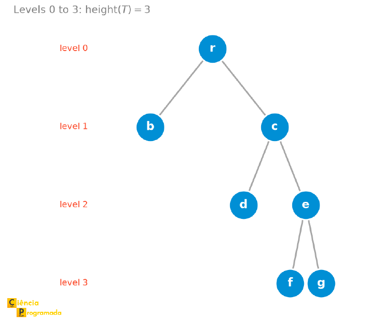
Solution:
- \(\text{level}(r) = 0\)
- \(\text{level}(b) = \text{level}(c) = 1\)
- \(\text{level}(d) = \text{level}(e) = 2\)
- \(\text{level}(f) = \text{level}(g) = 3\)
- \(\text{height}(T) = 3\)
Recursion: computing the height programmatically
The definition of height (“the greatest level among all vertices”) is natural to compute top-down (from the root to the leaves), but the most direct way to program it is precisely the opposite: a recursive bottom-up function, which asks for the height of each child before answering for itself.
Representing the tree as a dictionary of children (the simplest way to store a rooted tree in Python), the height of a vertex is 0 if it has no children (it is a leaf), or 1 plus the greatest height among its children, otherwise:
children = {
    "r": ["b", "c"],
    "b": [],
    "c": ["d", "e"],
    "d": [],
    "e": ["f", "g"],
    "f": [],
    "g": [],
}

def height(node):
    if not children[node]:
        return 0
    return 1 + max(height(child) for child in children[node])

for node in children:
    print(f"height({node}) = {height(node)}")
height(r) = 3
height(b) = 0
height(c) = 2
height(d) = 0
height(e) = 1
height(f) = 0
height(g) = 0Note that height(r) = 3 is exactly the height of the entire tree \(T\)
(the root recursively “asks” for the height of the whole structure below
it), and that height(b) = height(d) = height(f) = height(g) = 0 for all
the leaves, which matches the fact that the level of a leaf is the greatest
“local” level of its own subtree (which is just itself). This is the same
recursive idea behind almost every algorithm that processes trees: solve
the problem on the subtrees first, and then combine the answers at the root.
These concepts appear everywhere in computer science: whenever a structure organizes data hierarchically, there is a rooted tree under the hood. The most literal example of all is precisely the one that opened this article: a file system.
Application: the tree behind a file system
Every file system is a rooted tree: the root is the main folder, each folder
is the child of exactly one parent folder, and files are the leaves. Let us
build a small real project structure (in a temporary folder, so the code
runs on any machine) and compute its levels and its height with networkx:
import os
import tempfile
from pathlib import Path

import networkx as nx

with tempfile.TemporaryDirectory() as tmp:
    root = Path(tmp) / "project"
    (root / "src").mkdir(parents=True)
    (root / "tests").mkdir()
    (root / "src" / "main.py").touch()
    (root / "src" / "utils.py").touch()
    (root / "tests" / "test_main.py").touch()
    (root / "README.md").touch()

    G = nx.Graph()
    for current_folder, subdirs, files in os.walk(root):
        current_folder = Path(current_folder)
        for name in subdirs + files:
            source = str(current_folder.relative_to(root.parent))
            target = str((current_folder / name).relative_to(root.parent))
            G.add_edge(source, target)

    print("Is it a tree?", nx.is_tree(G))
    levels = nx.shortest_path_length(G, root.name)
    for node, level in sorted(levels.items(), key=lambda x: (x[1], x[0])):
        print(f"level({node}) = {level}")
    print("height(project) =", max(levels.values()))
Is it a tree? True
level(project) = 0
level(project/README.md) = 1
level(project/src) = 1
level(project/tests) = 1
level(project/src/main.py) = 2
level(project/src/utils.py) = 2
level(project/tests/test_main.py) = 2
height(project) = 2os.walk traverses the directory tree from top to bottom, exactly as we did
by hand in the previous examples, only now on a real file structure, with
pathlib taking care of the paths. Each folder or file nested one level
deeper increases the “level” by 1, and the height of the tree is, as always,
the greatest of these values.
Rooted trees in computing
- Binary search tree: each node has at most 2 children; node in the left subtree < node < node in the right subtree
- Heap: nearly complete binary tree; parent node ≥ children (max-heap) or parent node ≤ children (min-heap)
- Trie: tree for storing strings, with paths from the root to each node representing prefixes
- Decision tree: used in machine learning; each internal node represents a decision condition, and the level at which it appears reflects its order of evaluation
Exercises #
The exercises below are in increasing order of difficulty: the first two reinforce the basic properties of trees and forests, and the third revisits the spanning tree from the previous example.
Exercise 1: Number of edges
Statement: How many edges does a forest with 10 vertices and 3 connected components have?
Solution
Each connected component with \(n_i\) vertices is a tree with \(n_i - 1\) edges. If the components have \(n_1, n_2, n_3\) vertices with \(n_1 + n_2 + n_3 = 10\), the total number of edges is \((n_1 - 1) + (n_2 - 1) + (n_3 - 1) = 10 - 3 = 7\) edges.
Exercise 2: Uniqueness of the path
Statement: In a tree with 6 vertices forming the path \(1 - 2 - 3 - 4 - 5 - 6\) with an extra edge \(\{2, 5\}\), is the resulting graph still a tree?
Solution
No. The graph has 6 vertices and 6 edges (the path has 5 + the extra edge = 6). A tree with 6 vertices has exactly 5 edges. Besides, there is a cycle: \(2 - 3 - 4 - 5 - 2\). Therefore, it is not a tree.
Exercise 3: another order, another spanning tree
Statement: Revisit the graph \(G\) with the edge list \(\{(a,b), (a,c), (b,c), (c,e), (a,e), (e,f), (a,f), (e,d), (c,d)\}\) from Example 2 of the spanning tree section. Choose a different order for this edge list and find a spanning tree of \(G\) different from the one obtained earlier.
Solution
For example, going through the edges in the order \((a,e), (e,f), (e,d), (a,b), (a,c), (c,e), (b,c), (a,f), (c,d)\), accepting each edge that does not close a cycle with those already chosen, we obtain the edge set \(\{(a,e), (e,f), (e,d), (a,b), (a,c)\}\), which already connects the 6 vertices with exactly 5 edges: a spanning tree different from that of Example 2. Any other order that yields a tree with the same properties (connected, acyclic, 5 edges, 6 vertices) is also correct; the important thing is to realize that the order in which edges are chosen determines which specific spanning tree you get.
Summary #
| Concept | Description |
|---|---|
| Tree | Connected and acyclic graph |
| Forest | Acyclic graph (each component is a tree) |
| Leaf | Vertex of degree 1 |
| Theorem 1 | There is a unique path between each pair of vertices \(\Leftrightarrow\) the graph is a tree |
| Theorem 2 (\(m = n-1\)) | Every tree with \(n\) vertices has \(n-1\) edges |
| Eccentricity / Center | \(e(v) = \max_w d(v,w)\); \(c(G)\) = vertices of minimum eccentricity |
| Center of a tree | 1 vertex, or 2 adjacent vertices; found by iteratively removing leaves |
| Balanced tree | Subtrees of each vertex with similar sizes (in AVL trees, heights that differ by at most 1); logarithmic height |
| Spanning tree | Spanning subgraph that is a tree; in general not unique |
| Root | Special vertex in rooted trees |
| Ancestor / Descendant / Parent / Child | Relations defined by the unique path from the root to each vertex |
| Level / Height | \(\text{level}(v)\) = length of the path from the root to \(v\); \(\text{height}(T) = \max_v \text{level}(v)\) |
Next Steps #
Trees are the minimal skeleton that keeps a graph connected, but, because they are acyclic, they cannot answer questions about graphs that do have cycles and where we want to traverse the whole structure in some specific way: visiting each edge exactly once, or visiting each vertex exactly once. These questions motivate Eulerian and Hamiltonian graphs, the topic of the next article in the series: Eulerian trails (which traverse all the edges of a graph) and Hamiltonian cycles (which visit all the vertices), including the traveling salesman problem.


