

Two graphs can have vertices with different names and still be, in essence, exactly the same. Imagine a subway map drawn in two different ways: the stations have different labels on paper, but the connections between them are the same. Mathematically, these two graphs are isomorphic.
In this article, we formalize this notion and also study how to represent graphs so that computers can work with them: adjacency matrices and incidence matrices.
Why Do Isomorphism and Matrix Representation Matter? #
- Chemistry: two molecules can be described by different graphs (atoms numbered in different ways) and still be the same substance, and deciding that is deciding a graph isomorphism.
- Circuit verification: two circuit schematics drawn in different ways can represent exactly the same network of components.
- Compilers and optimization: equivalent control-flow graphs, produced by different compilation paths, must be recognized as “the same graph” so that the same optimizations can be applied.
- Data structures in software: graph libraries must choose how to store a graph
in memory.
networkx, in Python, uses adjacency lists (dictionaries of neighbors) and produces the adjacency or incidence matrix when asked; numerical libraries work directly with matrices. Understanding these representations is understanding how the computer really “sees” a graph. - Linear algebra applied to networks: eigenvalues and eigenvectors of the adjacency matrix (the “spectrum” of the graph) are used in algorithms such as PageRank and in social network analysis.
Graph Isomorphism #
Same Graph, Different Drawings #
Before defining isomorphism formally, it is worth seeing the phenomenon in practice: very different geometric representations can correspond to exactly the same graph (same vertex set, same edge set).
Example: two representations of the same graph
Statement: Let \(G\) be the graph with \(V(G) = \{a,b,c,d,e\}\) and \(E(G) = \{(a,b), (b,c), (a,c), (a,e), (c,d), (e,d)\}\). Do the two geometric representations below show the same graph?
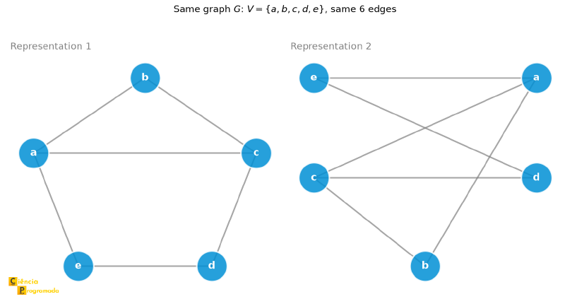
Solution: Yes. The two figures have completely different vertex positions, but they describe exactly the same graph: same vertices, same edges.
Example: \(K_4\) in three representations
Statement: The complete graph \(K_4\) (vertices \(\{1,2,3,4\}\), all \(\binom{4}{2} = 6\) possible edges) can be drawn in visually very different ways. Do the three figures below represent the same graph?
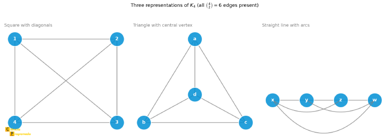
Solution: Yes. At first sight the three figures look like different graphs, but all of them represent \(K_4\).
Similar Drawings, Different Graphs #
The converse also happens: two drawings can look practically identical and still correspond to formally different graphs.
Example: \(H_1\) and \(H_2\)
Statement: Let \(H_1\) and \(H_2\) be two graphs with the same vertex set \(V(H_1) = V(H_2) = \{1,2,a,b\}\), but with
$$E(H_1) = \{(1,a), (1,b), (2,a), (2,b)\}$$$$E(H_2) = \{(1,a), (1,2), (b,a), (b,2)\}$$Are \(H_1\) and \(H_2\) the same graph? Are they isomorphic?
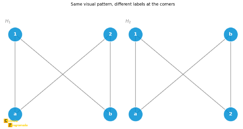
Solution: The two drawings have the same visual crossing pattern, but \(E(H_1) \neq E(H_2)\) as sets of pairs with the same labels, so \(H_1\) and \(H_2\) are formally different graphs.
Curiously, if we rename the vertices of \(H_2\) by swapping \(b\) with \(2\) and \(2\) with \(b\), we obtain exactly \(H_1\). That is, \(H_1\) and \(H_2\) are not the same graph, but they are isomorphic to each other, a notion we will formalize next.
The Isomorphism Problem #
The examples above raise a natural question: given two geometric representations of graphs, do they correspond to the same graph (up to renaming vertices)? In other words, is it possible to associate each point of one representation with a point of the other so as to preserve adjacencies, that is, so that the edges coincide?
This question has a name: the Graph Isomorphism Problem. The formal definition below is the precise answer to this question.
Two graphs \(G_1\) and \(G_2\) are isomorphic, denoted \(G_1 \approx G_2\), when there exists a bijective function (injective and surjective)
$$f: V(G_1) \to V(G_2)$$such that:
$$(v, w) \in E(G_1) \iff (f(v), f(w)) \in E(G_2)$$In words: \(f\) is a bijection between the vertices that preserves adjacencies, that is, two vertices are adjacent in \(G_1\) if and only if their images are adjacent in \(G_2\). The function \(f\) is called an isomorphism between \(G_1\) and \(G_2\).
Necessary (But Not Sufficient) Conditions #
From the definition itself we can already deduce mandatory consequences of \(G_1 \approx G_2\). For \(G_1 \approx G_2\), the following conditions are necessary:
- \(|V(G_1)| = |V(G_2)|\) (same number of vertices), a direct consequence of \(f\) being injective and surjective.
- \(|E(G_1)| = |E(G_2)|\) (same number of edges), because for each pair \((v,w) \in E(G_1)\) there is a corresponding pair \((f(v), f(w)) \in E(G_2)\), and since \(f\) is bijective this correspondence is also a bijection between the edges.
- The degree sequences of \(G_1\) and \(G_2\) are equal: since \(f\) preserves adjacencies vertex by vertex, the degree of \(v\) in \(G_1\) equals the degree of \(f(v)\) in \(G_2\).
The conditions above are necessary, but not sufficient. Two graphs can satisfy all of them and still not be isomorphic, as the counterexample below shows.
The problem of deciding whether two graphs are isomorphic (the Graph Isomorphism Problem) is one of the great open problems of computational complexity theory: it is not known whether it is in P (the class of problems solvable in polynomial time), but it has not been proved NP-complete either. A problem is NP-complete when it is among the hardest in the class NP (short for nondeterministic polynomial time, the class of problems whose solution, once found, can be verified quickly): every other problem in NP can be reduced to it in polynomial time, so that if someone found a fast algorithm for an NP-complete problem, they would have a fast algorithm for all problems in NP.
This undefined status is rare among natural problems in NP. In 2015, László Babai announced a quasipolynomial-time algorithm, of the order of \(2^{O((\log n)^c)}\) for some constant \(c\), much faster than any exponential algorithm, although still not polynomial. In January 2017, Harald Helfgott found a flaw in the proof; Babai fixed it within a few days and the result stood (see the entry Graph isomorphism problem).
When the Necessary Conditions Are Not Enough #
Let us start with the easy case: when the necessary conditions already fail, the answer is immediate.
Example: non-isomorphic graphs (easy case)
Statement: Let \(G_1\) be the path \(P_4\), with degree sequence \((1,1,2,2)\), and \(G_2\) the star graph \(K_{1,3}\), with degree sequence \((1,1,1,3)\). Are \(G_1\) and \(G_2\) isomorphic?
Solution: No. Both have 4 vertices and 3 edges, but the degree sequences are different. Hence \(G_1 \not\approx G_2\).
Now the hard case, the reason the warning box above exists: two graphs can satisfy all the necessary conditions seen so far and still not be isomorphic.
Counterexample: when the necessary conditions mislead
Statement: Let \(G_1\) and \(G_2\) be the graphs below.
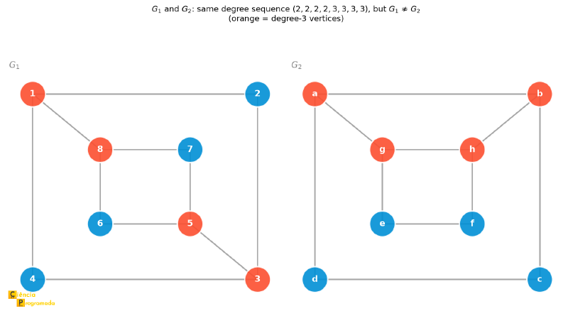
$$\begin{aligned}E(G_1) = \{&(1,2),(2,3),(3,4),(1,4),(8,7),\\ &(7,5),(5,6),(6,8),(1,8),(3,5)\}\end{aligned}$$$$V(G_2) = \{a,b,c,d,e,f,g,h\}$$
$$\begin{aligned}E(G_2) = \{&(a,b),(b,c),(c,d),(d,a),(g,h),\\ &(h,f),(f,e),(e,g),(a,g),(b,h)\}\end{aligned}$$
Are \(G_1\) and \(G_2\) isomorphic?
Solution: First, we check the necessary conditions: \(|V(G_1)| = |V(G_2)| = 8\), \(|E(G_1)| = |E(G_2)| = 10\), and the degree sequences of both are \((2,2,2,2,3,3,3,3)\). Everything matches! We are tempted to conclude that \(G_1 \approx G_2\).
But looking more carefully at how the degree-3 vertices connect to each other:
- In \(G_1\), vertex \(1\) (degree 3) is adjacent to \(2\) (degree 2), \(4\) (degree 2) and \(8\) (degree 3), and each degree-3 vertex is adjacent to two degree-2 vertices and one degree-3 vertex.
- In \(G_2\), vertex \(a\) (degree 3) is adjacent to \(b\) (degree 3), \(d\) (degree 2) and \(g\) (degree 3), and each degree-3 vertex is adjacent to two degree-3 vertices and one degree-2 vertex, the opposite pattern!
Since this local adjacency structure is different, no bijection can preserve all adjacencies simultaneously. Hence \(G_1 \not\approx G_2\), even though they satisfy all the necessary conditions seen so far. This is exactly what it means to say that these conditions are not sufficient.
Proving an Isomorphism #
After seeing that checking the necessary conditions can be misleading, the only reliable way to guarantee that \(G_1 \approx G_2\) is to explicitly exhibit a bijection \(f\) and verify that it preserves all adjacencies.
Example: proving \(G_1 \approx G_2\)
Statement: Let \(G_1\) and \(G_2\) be the graphs below, given by their geometric representation.
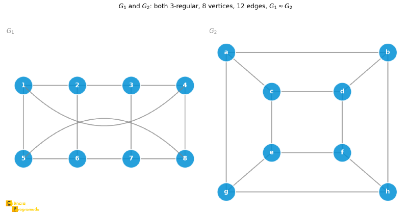
$$\begin{aligned}E(G_1) = \{&(1,2),(2,3),(3,4),(1,4),(5,6),(6,7),\\ &(7,8),(5,8),(1,5),(2,6),(3,7),(4,8)\}\end{aligned}$$$$V(G_2) = \{a,b,c,d,e,f,g,h\}$$
$$\begin{aligned}E(G_2) = \{&(a,b),(b,h),(h,g),(g,a),(c,d),(d,f),\\ &(f,e),(e,c),(a,c),(b,d),(g,e),(h,f)\}\end{aligned}$$
Are \(G_1\) and \(G_2\) isomorphic?
Solution: Before trying to prove that they are isomorphic, it is worth checking the necessary conditions: \(|V(G_1)| = |V(G_2)| = 8\), \(|E(G_1)| = |E(G_2)| = 12\), and both are 3-regular (every vertex has degree 3). The conditions match, but this only tells us that an isomorphism may exist, not that it does.
To prove that it exists, we exhibit the bijection \(f: V(G_1) \to V(G_2)\):
| \(v\) | \(f(v)\) |
|---|---|
| 1 | a |
| 2 | c |
| 3 | d |
| 4 | b |
| 5 | g |
| 6 | e |
| 7 | f |
| 8 | h |
It suffices to check that each of the 12 edges of \(G_1\) maps to an actual edge of \(G_2\). For example: \((1,2) \in E(G_1)\) and \((f(1),f(2)) = (a,c) \in E(G_2)\); \((1,4) \in E(G_1)\) and \((f(1),f(4)) = (a,b) \in E(G_2)\); \((1,5) \in E(G_1)\) and \((f(1),f(5)) = (a,g) \in E(G_2)\); and so on for the remaining edges. All of them check out, hence \(G_1 \approx G_2\).
The most natural procedure to decide whether two graphs with \(n\) vertices are isomorphic would be brute force: examine each of the \(n!\) possible permutations of vertices (that is, test each candidate bijective function) until finding one that preserves adjacencies, or exhausting all of them without success. The problem is that \(n!\) grows very fast: for \(n = 20\) there are already more than \(2 \times 10^{18}\) permutations. That is why the Graph Isomorphism Problem is considered computationally hard in practice, even without a definite status in complexity theory.
Adjacency Matrix #
For computer algorithms to process graphs, we need numerical representations. The most natural one is the adjacency matrix.
Given a graph \(G\) with \(n\) vertices \(V = \{v_1, v_2, \ldots, v_n\}\), the adjacency matrix \(A = (a_{ij})\) is an \(n \times n\) matrix where:
$$a_{ij} = \begin{cases} 1 & \text{if } (v_i, v_j) \in E(G) \\ 0 & \text{otherwise} \end{cases}$$
Example: adjacency matrix of a graph with 5 vertices
Statement: Write the adjacency matrix of the graph \(G\) with
$$V(G) = \{v_1, v_2, v_3, v_4, v_5\}$$$$E(G) = \{(v_1,v_2), (v_1,v_3), (v_1,v_5), (v_2,v_3), (v_3,v_4), (v_4,v_5)\}$$
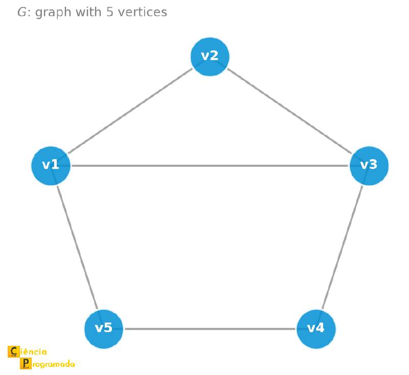
Solution:
$$A = \begin{pmatrix} 0 & 1 & 1 & 0 & 1 \\ 1 & 0 & 1 & 0 & 0 \\ 1 & 1 & 0 & 1 & 0 \\ 0 & 0 & 1 & 0 & 1 \\ 1 & 0 & 0 & 1 & 0 \end{pmatrix}$$Properties of the adjacency matrix of a simple graph:
- The main diagonal is all zeros: \(a_{ii} = 0\) (no loops)
- The matrix is symmetric: \(a_{ij} = a_{ji}\) (since edges are unordered pairs, in undirected graphs)
- The number of 1’s equals \(2m\), where \(m = |E(G)|\) (each edge \((v_i,v_j)\) contributes a 1 at \(a_{ij}\) and another at \(a_{ji}\))
- An adjacency matrix uniquely characterizes a graph, but the same graph can have several different adjacency matrices: just permute the order in which the vertices are listed.
Example: permuting the order of the vertices
Statement: Reorder the vertices of the graph in the previous example from \((v_1,v_2,v_3,v_4,v_5)\) to \((v_3,v_2,v_5,v_1,v_4)\) and write the new adjacency matrix.
Solution:
$$A' = \begin{pmatrix} 0 & 1 & 0 & 1 & 1 \\ 1 & 0 & 0 & 1 & 0 \\ 0 & 0 & 0 & 1 & 1 \\ 1 & 1 & 1 & 0 & 0 \\ 1 & 0 & 1 & 0 & 0 \end{pmatrix}$$Visually, \(A\) and \(A^{\prime}\) are different matrices, but both represent exactly the same graph.
The adjacency matrix holds more information than it seems: the entry \((A^k)_{ij}\) of the \(k\)-th power of \(A\) equals the number of walks of length \(k\) between \(v_i\) and \(v_j\). It is one of the reasons this representation is used in graph algorithms.
Incidence Matrix #
An alternative representation is the incidence matrix, which relates vertices to edges.
Given a graph \(G\) with \(n\) vertices and \(m\) edges, the incidence matrix \(B = (b_{ij})\) is an \(n \times m\) matrix where:
$$b_{ij} = \begin{cases} 1 & \text{if vertex } v_i \text{ is an endpoint of edge } e_j \\ 0 & \text{otherwise} \end{cases}$$
Example: incidence matrix of the same graph
Statement: Write the incidence matrix of the 5-vertex graph from the previous example, now with labeled edges: \(e_1=(v_1,v_2)\), \(e_2=(v_1,v_3)\), \(e_3=(v_2,v_3)\), \(e_4=(v_3,v_4)\), \(e_5=(v_4,v_5)\), \(e_6=(v_1,v_5)\).
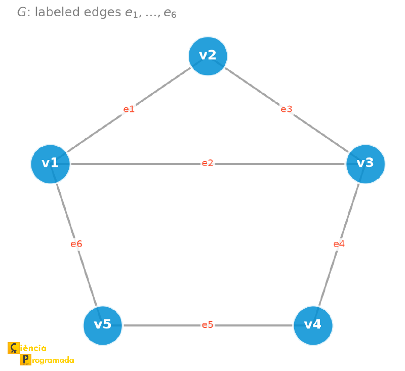
Solution:
$$B = \begin{array}{c|cccccc} & e_1 & e_2 & e_3 & e_4 & e_5 & e_6 \\ \hline v_1 & 1 & 1 & 0 & 0 & 0 & 1 \\ v_2 & 1 & 0 & 1 & 0 & 0 & 0 \\ v_3 & 0 & 1 & 1 & 1 & 0 & 0 \\ v_4 & 0 & 0 & 0 & 1 & 1 & 0 \\ v_5 & 0 & 0 & 0 & 0 & 1 & 1 \end{array}$$Row sums: \(d(v_1)=3, d(v_2)=2, d(v_3)=3, d(v_4)=2, d(v_5)=2\). Sum of all entries: \(12 = 2 \times 6\) edges.
Properties of the incidence matrix of a simple graph:
- Each column has exactly two 1s (each edge has two endpoints)
- The sum of row \(i\) equals \(d(v_i)\) (the degree of the vertex)
- The sum of all entries is \(2|E|\), which confirms the Handshaking Theorem
- An incidence matrix uniquely characterizes a graph, but the same graph can have several different incidence matrices: just permute the order of the vertices and/or the order of the edges.
Example: permuting vertices and edges
Statement: Simultaneously permute \((v_1,v_2,v_3,v_4,v_5) \to (v_3,v_5,v_1,v_4,v_2)\) and \((e_1,\ldots,e_6) \to (e_5,e_3,e_2,e_1,e_6,e_4)\) and write the new incidence matrix.
Solution:
$$B' = \begin{array}{c|cccccc} & e_5 & e_3 & e_2 & e_1 & e_6 & e_4 \\ \hline v_3 & 0 & 1 & 1 & 0 & 0 & 1 \\ v_5 & 1 & 0 & 0 & 0 & 1 & 0 \\ v_1 & 0 & 0 & 1 & 1 & 1 & 0 \\ v_4 & 1 & 0 & 0 & 0 & 0 & 1 \\ v_2 & 0 & 1 & 0 & 1 & 0 & 0 \end{array}$$Rows and columns in a different order, but still the same graph, exactly as happened with the adjacency matrix.
The Isomorphism Problem via Matrices #
Now that we know how to represent graphs numerically, the Isomorphism Problem can be restated in terms of matrices: given two \(n \times n\) adjacency matrices (or two \(n \times m\) incidence matrices), do they represent the same graph? It is the same question from the beginning of the article (remember the subway map redrawn with different labels?), only now applied to numerical representations instead of geometric ones. And it suffers from exactly the same difficulty: it is not enough to compare the matrices entry by entry, we must find out whether there is some permutation of rows and columns that turns one into the other.
Summary Table #
The table below summarizes the central definitions, conditions and properties presented in this article.
| Concept | Notation / Formula | Description |
|---|---|---|
| Isomorphism | \(G_1 \approx G_2\) if \(\exists f: V(G_1) \to V(G_2)\) bijective with \((v,w) \in E(G_1) \iff (f(v),f(w)) \in E(G_2)\) | \(f\) preserves adjacencies |
| Necessary conditions | \(\lvert V(G_1)\rvert = \lvert V(G_2)\rvert\), \(\lvert E(G_1)\rvert = \lvert E(G_2)\rvert\), same degree sequence | Necessary, not sufficient |
| Adjacency matrix | \(A = (a_{ij})\), \(n \times n\), \(a_{ij} = 1\) if \((v_i,v_j) \in E\) | Zero diagonal, symmetric, number of 1’s \(= 2m\), not unique (vertex permutation) |
| Incidence matrix | \(B = (b_{ij})\), \(n \times m\), \(b_{ij} = 1\) if \(v_i\) is an endpoint of \(e_j\) | Each column with two 1’s, sum of row \(i\) \(= d(v_i)\), total sum \(= 2\lvert E\rvert\), not unique (vertex and edge permutation) |
| Powers of the adjacency matrix | \((A^k)_{ij}\) | Number of walks of length \(k\) between \(v_i\) and \(v_j\) |
Comparing the Representations #
Besides knowing how to build each matrix, it is worth directly comparing the practical cost of using them in an algorithm:
| Aspect | Adjacency Matrix | Incidence Matrix |
|---|---|---|
| Dimension | \(n \times n\) | \(n \times m\) |
| Symmetry | Symmetric (undirected graph) | Not applicable (matrix is not square) |
| Check adjacency | \(O(1)\) | \(O(m)\) |
| List neighbors of \(v\) | \(O(n)\) | \(O(m)\) |
| Memory usage | \(O(n^2)\) | \(O(nm)\) |
For dense graphs (many edges), the adjacency matrix is usually more efficient. For sparse graphs, representations that store only the neighbors of each vertex (the so-called adjacency lists, one list per vertex instead of a full \(n \times n\) matrix of zeros) are preferable in practice.
Exercises #
Exercise 1: Isomorphism
Are the graphs \(G_1\) (a triangle plus an isolated vertex: \(K_3 \cup K_1\)) and \(G_2\) (the path \(P_4\)) isomorphic?
Solution
No. The degree sequence of \(G_1\) is \((0, 2, 2, 2)\) and that of \(G_2\) is \((1, 1, 2, 2)\). Since the sequences are different, \(G_1 \not\approx G_2\). \(\blacksquare\)
Exercise 2: Adjacency matrix
Write the adjacency matrix of the cycle \(C_5\) with vertices \(\{1, 2, 3, 4, 5\}\) and edges \((1,2), (2,3), (3,4), (4,5), (5,1)\).
Solution
All vertices have degree 2 (each row sums to 2), confirming that \(C_5\) is 2-regular. \(\blacksquare\)
Exercise 3: Incidence matrix
Let \(G\) be the graph “triangle with a pendant edge”: \(V(G) = \{p,q,r,s\}\), \(E(G) = \{(p,q), (q,r), (p,r), (r,s)\}\). Write the incidence matrix \(B\) of \(G\) and confirm that the sum of each row matches the degree of the corresponding vertex.
Solution
Labeling \(e_1=(p,q)\), \(e_2=(q,r)\), \(e_3=(p,r)\), \(e_4=(r,s)\):
$$B = \begin{array}{c|cccc} & e_1 & e_2 & e_3 & e_4 \\ \hline p & 1 & 0 & 1 & 0 \\ q & 1 & 1 & 0 & 0 \\ r & 0 & 1 & 1 & 1 \\ s & 0 & 0 & 0 & 1 \end{array}$$Row sums: \(d(p)=2, d(q)=2, d(r)=3, d(s)=1\), and they match exactly the degrees of each vertex in \(G\). \(\blacksquare\)
Exercise 4: Isomorphism via matrices
The adjacency matrices below represent, respectively, the graphs \(G_1\) (vertices \(1,2,3,4\)) and \(G_2\) (vertices \(a,b,c,d\)):
$$A_1 = \begin{pmatrix} 0 & 1 & 0 & 1 \\ 1 & 0 & 1 & 0 \\ 0 & 1 & 0 & 1 \\ 1 & 0 & 1 & 0 \end{pmatrix} \qquad A_2 = \begin{pmatrix} 0 & 1 & 1 & 0 \\ 1 & 0 & 0 & 1 \\ 1 & 0 & 0 & 1 \\ 0 & 1 & 1 & 0 \end{pmatrix}$$Are \(G_1\) and \(G_2\) isomorphic?
Solution
Yes, although they are not the same graph (the vertices have different names). \(A_1\) describes the cycle \(1-2-3-4-1\), and \(A_2\) describes the cycle \(a-b-d-c-a\) (check: \(a\) is adjacent to \(b\) and \(c\); \(b\) is adjacent to \(a\) and \(d\); etc.). The bijection \(f(1)=a, f(2)=b, f(3)=d, f(4)=c\) preserves all adjacencies, hence \(G_1 \approx G_2\). \(\blacksquare\)
Next Steps #
Isomorphism and matrices answer one specific question: given two entire graphs, are they “the same”? But neither of these tools tells us how to move within a single graph: what the route between two vertices is, when that route forms a cycle, or whether the whole graph is connected. These are the questions of the next article in the series: paths, cycles and connectivity.


