

How do we know whether two points of a network are connected, and by which shortest path? So far we have studied graphs as static objects, sets of vertices and edges. But the most common question about a graph is how to navigate it: starting from a vertex and following edges to reach others.
This leads us to the concepts of walks, trails, paths, and cycles, and to the notion of connectivity.
Why Do Paths and Cycles Matter? #
Navigating a graph, and knowing whether that navigation is even possible, is the basis of central problems in computer science and applied mathematics:
- Network routing: routing protocols (such as those used on the internet) need to find paths between routers, and the concept of shortest distance directly defines the cost of a route.
- Distributed systems: before running any distributed algorithm, it is common to check whether the network of machines is connected; if it is not, the system splits into partitions that cannot communicate.
- Resource allocation: matching problems (such as assigning workers to machines, or candidates to openings) are modeled as bipartite graphs, and solving them depends on understanding the structure of these graphs.
- Verification of circuits and protocols: detecting cycles in a dependency graph is what prevents, for example, deadlocks in concurrent systems or circular references in software builds.
Walks, Trails, and Paths #
There are different ways to traverse a graph, and the distinctions between them matter:
A walk in \(G\) is a sequence of vertices
$$P = v_0, v_1, \ldots, v_k$$such that \((v_i, v_{i+1}) \in E(G)\) for \(0 \leq i \leq k-1\), that is, between each pair of consecutive vertices of the sequence there is an edge of \(G\).
The integer \(k\) (the number of edges traversed) is the length of the walk, \(v_0\) is its start, \(v_k\) is its end, and we say that \(P\) is a walk from \(v_0\) to \(v_k\).
In a walk, vertices and edges may repeat.
A trail is a walk in which no edge repeats (but vertices may repeat).
A path is a walk in which no vertex repeats (and therefore no edge repeats either).
The hierarchy is: every path is a trail, and every trail is a walk. The converse is not necessarily true.
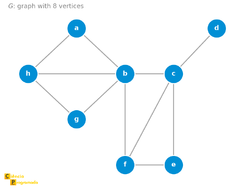
To fix these ideas, we will use the same graph \(G\) in several examples throughout this article, to observe how the same eight vertices support increasingly specific concepts, from walk to graph center. We start from the graph \(G\) below:
Example: walk, trail, and path in the same graph
Statement: In the graph \(G\) above, classify the sequences \(P_1 = a, b, c, d, c, b, g\), \(P_2 = a, b, c, f, b, g\), \(P_3 = a, h, g\), and \(P_4 = g, h, a, b, f, e, c, d\) as walk, trail, or path.
Solution:
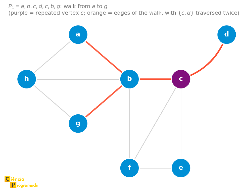
- \(P_1\) is a walk from \(a\) to \(g\): the vertices \(b\) and \(c\) and the edges \(\{b,c\}\) and \(\{c,d\}\) appear twice.
- \(P_2\) is a trail from \(a\) to \(g\): no edge repeats, but the vertex \(b\) appears twice, so \(P_2\) is not a path.
- \(P_3\) is a path between \(a\) and \(g\): no vertex repeats.
- \(P_4\) is also a path, now between \(g\) and \(d\), passing through all the other vertices of \(G\) without repeating any.
The figure below highlights \(P_1\) over the graph \(G\), showing where the vertex \(c\) and the edge \(\{c,d\}\) repeat:
Closed Walks and Closed Trails #
A walk (or trail, or path) is closed if the initial vertex coincides with the final vertex, that is, \(v_0 = v_k\).
A closed trail is a closed walk in which all edges are distinct.
A cycle is a closed walk in which, in addition, all vertices are distinct, except for the first and the last, which coincide by definition. In other words, if \(v_0 = v_k\) and \(v_0, v_1, \ldots, v_{k-1}\) is a path, then \(P\) is a cycle.
The length of a cycle is given by its number of edges (equal to its number of distinct vertices).
A cycle with an odd number of edges is called an odd cycle; otherwise, it is called an even cycle.
Cycles of length 3 are triangles.
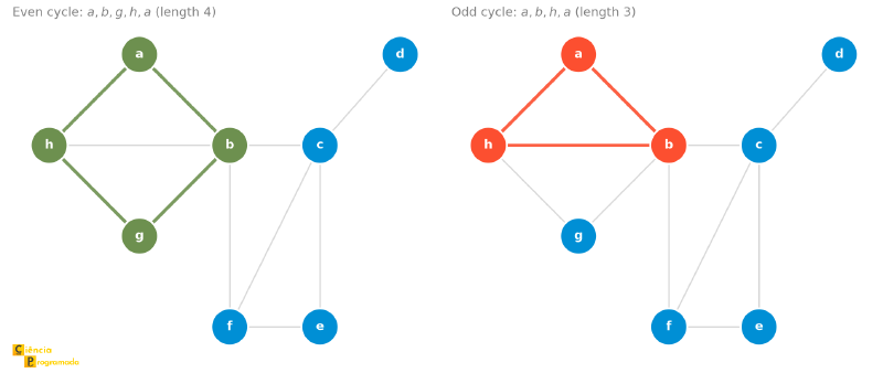
The graph \(G\) has examples of both kinds: a cycle of length 4 (\(a,b,g,h,a\)) and a triangle, which is a cycle of length 3 (\(a,b,h,a\)):
Example: closed walk, closed trail, and cycles
Statement: Still in the graph \(G\), classify \(P_5 = a, b, c, d, c, e, f, b, g, h, a\), \(P_6 = a, b, c, e, f, b, g, h, a\), \(P_7 = a, b, g, h, a\), and \(P_8 = a, b, h, a\).
Solution:
- \(P_5\) is a closed walk, but not a closed trail: the edge \(\{c,d\}\) is traversed twice.
- \(P_6\) is a closed trail (no edge repeats), but it is not a cycle, since the vertex \(b\) is visited twice.
- \(P_7\) is an even cycle, of length 4.
- \(P_8\) is an odd cycle, of length 3 (a triangle).
Application: detecting circular dependencies
Cycles show up (and cause headaches) whenever a software system models dependencies between components as a directed graph: if module \(A\) depends on \(B\), we draw an edge \(A \to B\). A project only compiles (or imports, or installs) if this dependency graph has no cycles; otherwise, “what to load first” becomes a question with no answer.
import networkx as nx

deps = nx.DiGraph()
deps.add_edges_from([
    ("app", "auth"),
    ("app", "database"),
    ("auth", "database"),
    ("database", "config"),
    ("config", "utils"),
    ("utils", "auth"),  # closes the cycle auth -> database -> config -> utils -> auth
])

try:
    cycle = nx.find_cycle(deps)
    print("Circular dependency found:")
    for source, target in cycle:
        print(f"  {source} -> {target}")
except nx.NetworkXNoCycle:
    print("No cycle: the dependency graph is a DAG, safe build.")
Circular dependency found:
auth -> database
database -> config
config -> utils
utils -> authThe graph below shows the declared dependencies, with the cycle found highlighted in orange:
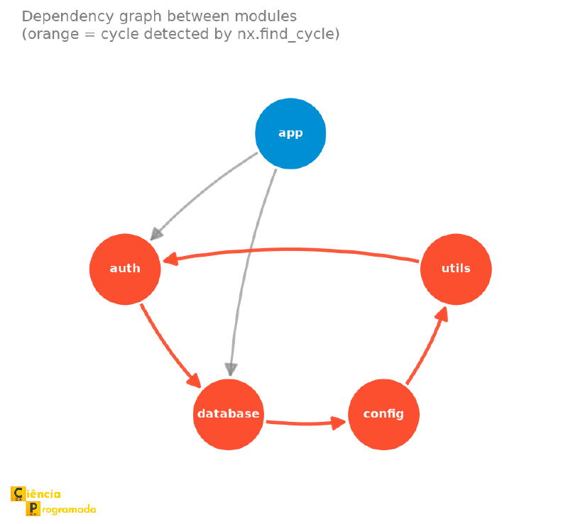
The cycle is not obvious when looking module by module: auth imports
database, which imports config, which imports utils, which in turn
imports auth back. This is exactly the kind of indirect circular
dependency that build systems and package managers such as pip and npm
traverse as a graph, instead of relying on someone to notice the problem
manually.
What each tool does when it finds a cycle varies: cargo (Rust) refuses
the build outright (it only accepts cycles between dev-dependencies), like
many compiled build systems, since compiling requires a strict order
between dependencies; classic make detects it, warns, and breaks the
cycle arbitrarily to move on; and interpreted languages such as Python and
Node.js tolerate the circular import at run time, handing over a partially
initialized module at the point where the cycle closes, a classic source of
subtle bugs. Behind all these strategies lies the same fact from graph
theory: a valid build, install, or import order is a
topological sort,
and a topological sort only exists if the directed graph is acyclic, which
is why these tools need to check whether sorting is even possible, even when
they decide to tolerate the cycle.
Connectivity #
So far we have said “there is a path between \(v\) and \(w\)” loosely. Let us formalize this idea pair by pair before applying it to the whole graph.
Two vertices \(v\) and \(w\) are connected in \(G\) when there is some path between \(v\) and \(w\) in \(G\).
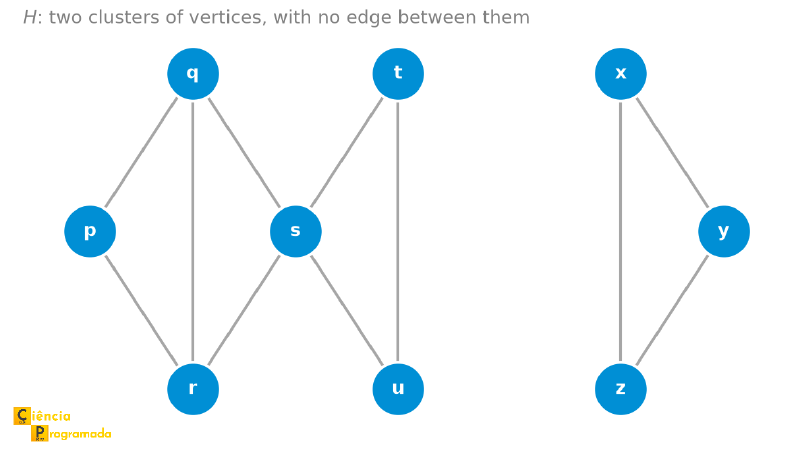
Now consider the graph \(H\) below, formed by a cluster of six vertices \(\{p,q,r,s,t,u\}\) and, separately, a triangle \(\{x,y,z\}\):
Example: checking connectivity pair by pair
Statement: In the graph \(H\), are \(p\) and \(t\) connected? And \(p\) and \(x\)?
Solution:
- \(p\) and \(t\) are connected: the path \(P = p, r, s, t\) links the two.
- \(p\) and \(x\) are not connected: there is no path between them, since no edge links the cluster \(\{p,\ldots,u\}\) to the triangle \(\{x,y,z\}\).
A graph \(G\) is connected when every pair of distinct vertices of \(G\) is connected, that is, when there is a path between any pair of vertices \(u, v \in V(G)\). Otherwise, \(G\) is disconnected.
The graph \(H\) of the example above is disconnected, but each of its two parts, on its own, is connected. This leads us to the definition of connected component.
Let \(G = (V, E)\) be a graph and \((V_1, V_2, \ldots, V_k)\) a partition of \(V\) (that is, \(V_1 \cup V_2 \cup \cdots \cup V_k = V\) and \(V_i \cap V_j = \emptyset\) for \(i \neq j\)). The induced subgraph \(G[V_i]\) is a connected component of \(G\) if:
- \(G[V_i]\) is connected, and
- for every vertex \(v \in V - V_i\), the subgraph \(G[V_i \cup \{v\}]\) is not connected.
Condition 2 is what forces each component to be the largest possible connected subgraph: if any outside vertex is added to \(V_i\), the result stops being connected. It is in this sense that connected components are the “maximal connected pieces” of \(G\).
We denote by \(\omega(G)\) the number of connected components of \(G\). A graph is connected if and only if \(\omega(G) = 1\).
\(\omega(G)\) for the number of components is common in Portuguese-language texts, but it is not universal: many English books write \(c(G)\) or \(k(G)\) and reserve \(\omega(G)\) for the clique number, the size of the largest clique of \(G\). It is worth checking the convention when consulting another source. In this article, \(c(G)\) is the center of the graph, defined later.
Many graph algorithms assume, as a precondition, that the input graph is connected. When that is not the case, a common step is to “preprocess” the graph to split it into its connected components and solve the problem in each one of them separately.
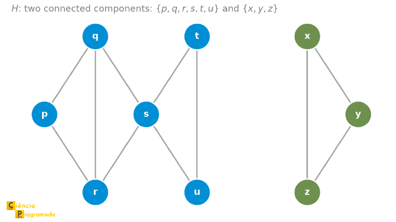
Back to the graph \(H\), we highlight its two connected components below:
Example: counting connected components
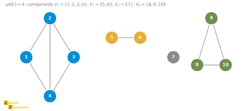
Statement: How many connected components does the graph \(H\) have? And a graph \(G^{\prime}\) with \(V(G^{\prime}) = \{1, \ldots, 10\}\) partitioned into \(V_1 = \{1,2,3,4\}\) (with edges \(\{1,2\},\{1,4\},\{2,3\},\{2,4\},\{3,4\}\)), \(V_2 = \{5,6\}\) (with the edge \(\{5,6\}\)), \(V_3 = \{7\}\) (isolated vertex), and \(V_4 = \{8,9,10\}\) (a triangle)?
Solution: In the graph \(H\), the subgraph induced by \(\{p,q,r,s,t,u\}\) is connected, and the subgraph induced by \(\{x,y,z\}\) is also connected, and no vertex can be moved from one to the other without breaking connectivity. Hence these are the two connected components of \(H\), and \(\omega(H) = 2\).
A graph can have many components, including isolated vertices. Each \(G^{\prime}[V_i]\) is connected and maximal, so \(\omega(G^{\prime}) = 4\).
The figure below shows \(G^{\prime}\), with each connected component in a different color:
And what about the graph \(G\) we saw in the previous section (vertices \(\{a,\ldots,h\}\))? Every pair of vertices of \(G\) is connected. For example, \(P_4\) already showed a path between \(g\) and \(d\) passing through all the other vertices. Hence \(G\) is connected and \(\omega(G) = 1\).
Distance, Eccentricity, and Diameter #
With the concept of connectivity in hand, we can measure “distances” within a graph:
The distance \(d(v, w)\) between two vertices \(v\) and \(w\) is the length of the shortest path between them, which is also called a geodesic. If \(v\) and \(w\) are not connected (that is, they are in distinct connected components of \(G\)), there is no path between them, and we define \(d(v,w) = \infty\).
The following definitions (eccentricity, diameter, and center) assume that \(G\) is a connected graph (otherwise, some \(e(v)\) could be infinite).
Let \(G\) be a connected graph. The eccentricity \(e(v)\) of a vertex \(v\) is the greatest distance from \(v\) to any other vertex:
$$e(v) = \max_{w \in V} d(v, w)$$The diameter of \(G\) is the greatest eccentricity:
$$\text{diam}(G) = \max_{v \in V} e(v) = \max_{v,w \in V} d(v,w)$$The center of \(G\) is the set of vertices with the smallest eccentricity:
$$c(G) = \{v \in V : e(v) = \min_{u \in V} e(u)\}$$Let us compute these three measures in the graph \(G\) (vertices \(\{a,\ldots,h\}\)) that we used in the previous sections.
Example: eccentricity, diameter, and center of \(G\)
Statement: Compute the eccentricity of each vertex of \(G\), the diameter of \(G\), and its center.
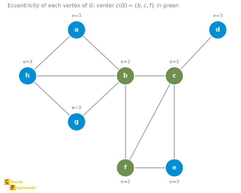
Solution: Starting from \(a\), the distances to the other vertices are: \(d(a,b)=1\), \(d(a,h)=1\), \(d(a,g)=2\), \(d(a,c)=2\), \(d(a,f)=2\), \(d(a,e)=3\), \(d(a,d)=3\). The greatest of them is 3, so \(e(a) = 3\).
Repeating the computation for all vertices of \(G\), we obtain:
$$e(a) = e(d) = e(e) = e(g) = e(h) = 3 \qquad e(b) = e(c) = e(f) = 2$$Since the greatest eccentricity is 3, we have \(\text{diam}(G) = 3\). And since \(b\), \(c\), and \(f\) are the vertices of smallest eccentricity (2), the center is \(c(G) = \{b, c, f\}\), exactly the three vertices that sit between the “left side” (\(a,g,h\)) and the “right side” (\(d,e\)) of \(G\), which makes intuitive sense: vertices through which the paths between the two parts of the graph pass tend to be closer to everyone.
The following figure shows the eccentricity of each vertex and highlights the center:
Example: the case of the path \(P_5\)
Statement: Compute the eccentricity of each vertex, the diameter, and the center of the path \(P_5 = v_1 - v_2 - v_3 - v_4 - v_5\).
Solution: In a path graph, the eccentricity grows quite predictably from the ends:
- \(e(v_1) = e(v_5) = 4\) (the ends must cross the whole path)
- \(e(v_2) = e(v_4) = 3\)
- \(e(v_3) = 2\) (the central vertex)
Diameter = 4. Center = \(\{v_3\}\). In any \(P_n\), the center is always the vertex (or vertices) closest to the middle of the sequence.
Checking with code
Everything we computed by hand for the graph \(G\) (eccentricities,
diameter, and center) comes out in a few lines with networkx:
import networkx as nx

G = nx.Graph()
G.add_edges_from([
    ("a","b"), ("a","h"), ("b","h"), ("b","g"), ("g","h"),
    ("b","c"), ("b","f"), ("c","f"), ("c","e"), ("e","f"), ("c","d"),
])

print("Eccentricities:", nx.eccentricity(G))
print("Diameter:", nx.diameter(G))
print("Center:", nx.center(G))
Eccentricities: {'a': 3, 'b': 2, 'h': 3, 'g': 3, 'c': 2, 'f': 2, 'e': 3, 'd': 3}
Diameter: 3
Center: ['b', 'c', 'f']The values match the manual computation exactly. Besides avoiding arithmetic mistakes, the same code works with no change for a graph with 8 or with 8 million vertices; what we did by hand for \(G\) is only feasible by hand because the graph is small.
Computing Distances: Breadth-First Search #
In the examples above, we read the distances off the drawing of \(G\), and
networkx did the same computation in one line. But how do we compute the
distance between two vertices of a graph with millions of them? When the
edges have no weights, the answer is breadth-first search (BFS).
The idea is to explore the graph in layers from a source \(v\): first \(v\) itself, at distance 0; then all its neighbors, at distance 1; then the neighbors of those neighbors that have not appeared yet, at distance 2; and so on. A queue guarantees this order: each discovered vertex enters at the rear of the queue, and vertices are processed in the order in which they entered.
Given a source vertex \(v\):
- Mark \(d(v, v) = 0\) and put \(v\) in the queue.
- While the queue is not empty, remove the first vertex \(u\) from the queue. For each neighbor \(w\) of \(u\) that does not yet have a distance marked, mark \(d(v, w) = d(v, u) + 1\) and put \(w\) at the rear of the queue.
At the end, each vertex reachable from \(v\) has its distance marked; those left unmarked are in another connected component, at distance \(\infty\).
Why is the marked distance the smallest possible? Vertices leave the queue in increasing order of distance (all those in layer \(k\) before any of layer \(k+1\)), so the first time a vertex \(w\) appears is from a vertex in the layer closest possible to the source. And the cost is low: each vertex enters the queue only once, and each edge is examined twice, once from each endpoint, which gives time \(O(n + m)\).
Applied to the graph \(G\) from \(a\), BFS reproduces the distances we computed by hand:
from collections import deque

import networkx as nx

G = nx.Graph()
G.add_edges_from([
    ("a", "b"), ("a", "h"), ("b", "h"), ("b", "g"), ("g", "h"),
    ("b", "c"), ("b", "f"), ("c", "f"), ("c", "e"), ("e", "f"), ("c", "d"),
])


def distances(G, source):
    """Distance from source to each reachable vertex, by breadth-first search."""
    dist = {source: 0}
    queue = deque([source])
    while queue:
        v = queue.popleft()
        for w in G.neighbors(v):
            if w not in dist:  # first time w appears
                dist[w] = dist[v] + 1
                queue.append(w)
    return dist


d_a = distances(G, "a")
print(d_a)
# Output: {'a': 0, 'b': 1, 'h': 1, 'g': 2, 'c': 2, 'f': 2, 'e': 3, 'd': 3}
print(max(d_a.values()))  # 3, the eccentricity of a
The figure below draws \(G\) in these layers. The thick edges are the ones the search used to discover each vertex; the dashed ones were examined and discarded, because the vertex on the other side already had a distance marked:
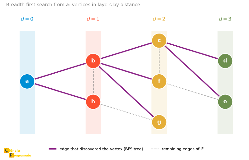
The greatest distance found is the eccentricity of \(a\). Running BFS from each vertex, we obtain all the eccentricities (and, with them, the diameter and the center) in time \(O(n(n + m))\). The same search comes back later in this article, to test whether a graph is bipartite, and in the article on trees, where it produces a spanning tree. It was described by Konrad Zuse in 1945, in a thesis that would only be published in 1972, and reinvented by Edward F. Moore in 1959 to find the way out of mazes (see the entry Breadth-first search).
Weighted graphs: Dijkstra’s algorithm
On a street map, edges have different lengths, and the path with the fewest edges is not always the shortest. In a weighted graph, each edge has a weight (distance, time, cost), and the length of a path becomes the sum of the weights of its edges. BFS, which only counts edges, no longer works.
Dijkstra’s algorithm, conceived by Edsger W. Dijkstra in 1956 and published in 1959, adapts the same idea: it swaps the ordinary queue for a priority queue and, at each step, fixes the distance of the not-yet-fixed vertex that is closest to the source. The algorithm requires nonnegative weights and, with the priority queue built on a heap, runs in time \(O((n + m) \log n)\). Routing apps use variations of it, with many optimizations for country-sized graphs.
In the graph below, the path with the fewest edges from \(A\) to \(B\) is the direct edge, of weight 4; the shortest one goes through \(C\) and \(D\) and has length 3:
import networkx as nx

G = nx.Graph()
G.add_weighted_edges_from([("A", "B", 4), ("A", "C", 1), ("C", "D", 1), ("D", "B", 1)])

print(nx.shortest_path(G, "A", "B"))         # ['A', 'B'] (unweighted: BFS)
print(nx.dijkstra_path(G, "A", "B"))         # ['A', 'C', 'D', 'B']
print(nx.dijkstra_path_length(G, "A", "B"))  # 3
Special Graphs #
Some graphs appear so frequently in applications and examples that it is worth naming them and recognizing them at once.
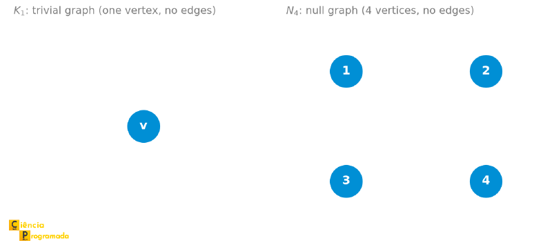
The complete graph \(K_n\) has \(n\) vertices, with every pair of vertices joined by an edge. In particular, \(K_1\), the complete graph on a single vertex, with no edges, is called the trivial graph.
The null graph \(N_n\) has \(n\) vertices and no edges, the opposite extreme of the complete graph.
The two extreme cases, side by side:
Cycles and Paths #
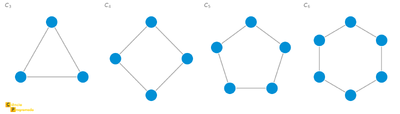
- \(C_n\): cycle with \(n\) vertices (\(n \geq 3\)), 2-regular
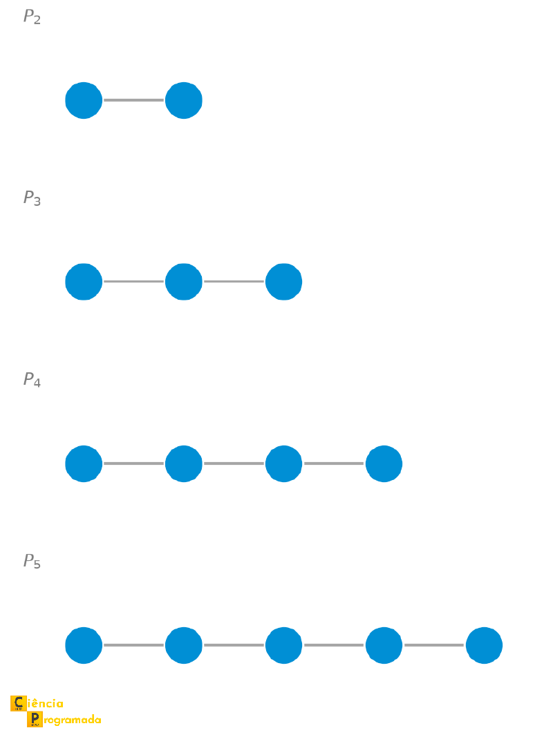
- \(P_n\): path with \(n\) vertices (\(n-1\) edges), with two vertices of degree 1 and \(n-2\) of degree 2
The first cycles of the family \(C_n\):
And the first paths of the family \(P_n\):
Bipartite Graphs #
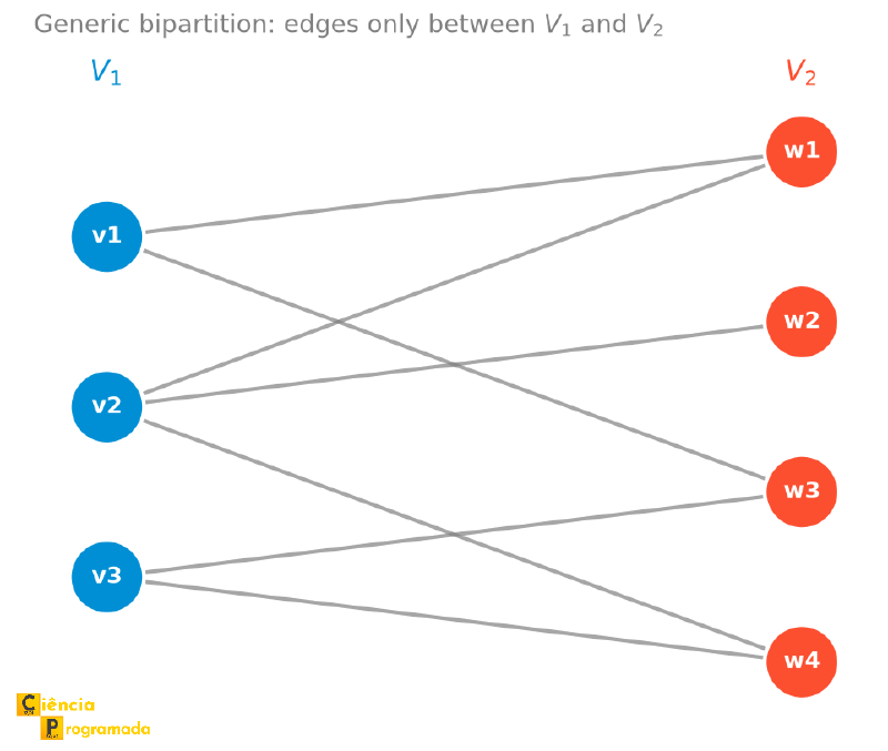
An important class of graphs is the one in which the vertices can be divided into two groups, with edges only between the groups.
A graph \(G = (V, E)\) is bipartite if \(V\) can be partitioned into two subsets \(V_1\) and \(V_2\) (with \(V_1 \cup V_2 = V\) and \(V_1 \cap V_2 = \emptyset\)) such that every edge of \(G\) has one endpoint in \(V_1\) and the other in \(V_2\). We say that \((V_1, V_2)\) is a bipartition of \(V\).
Since every edge links \(V_1\) to \(V_2\), there can be no edge between two vertices of \(V_1\), nor between two vertices of \(V_2\). That is, \(V_1\) and \(V_2\) are independent sets in \(G\). This observation will be useful to understand why cycles in bipartite graphs are always even, later on.
A useful way to visualize a bipartite graph is to draw \(V_1\) and \(V_2\) as two separate columns, making explicit that every edge crosses from one column to the other:
Example: assigning workers to machines
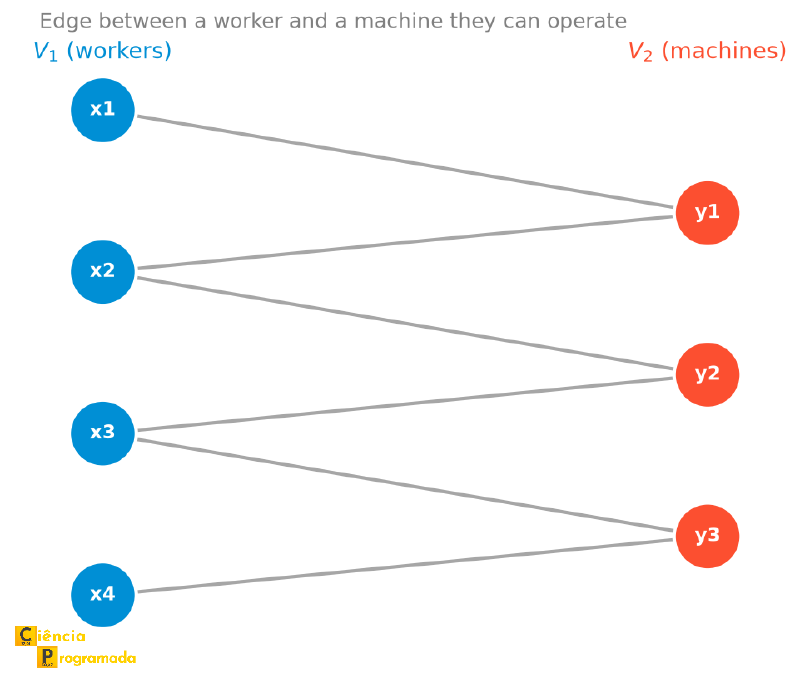
Statement: How do we model, as a bipartite graph, the problem of knowing which workers in a factory know how to operate which machines?
Solution: Let the workers \(x_1, x_2, \ldots, x_r\) form \(V_1\) and the machines \(y_1, y_2, \ldots, y_s\) form \(V_2\). There is an edge between worker \(x_i\) and machine \(y_j\) whenever \(x_i\) is able to operate \(y_j\). This graph is bipartite by construction: there is never an edge between two workers or between two machines, only between a worker and a machine. This is the kind of structure that matching problems exploit to decide, for example, who should operate what.
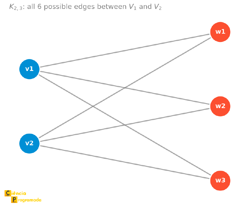
The complete bipartite graph \(K_{p,q}\) has \(|V_1| = p\), \(|V_2| = q\), and every possible edge between \(V_1\) and \(V_2\). Therefore, \(|E(K_{p,q})| = p \cdot q\).
A small example is \(K_{2,3}\), with all the \(2 \times 3 = 6\) possible edges between the two sides:
Examples of bipartite graphs:
- Paths \(P_n\) (for \(n \geq 2\)): even-position vertices in \(V_1\), odd-position ones in \(V_2\)
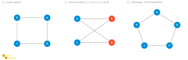
- Even cycles \(C_{2k}\): vertices alternating between \(V_1\) and \(V_2\)
The following figure shows \(C_4\) drawn in two ways (as a polygon and as a bipartition) and brings \(C_5\) as a challenge: try to find a valid bipartition for it (spoiler: there is none, as the next theorem will explain).
The complete bipartite graph \(K_{3,3}\) is the graph of the “three houses and three utilities problem”: three houses that must be connected to water, electricity, and gas without any line crossing. It is a classic example used to discuss graph planarity, the topic of an upcoming article in this series.
Characterization of Bipartite Graphs #
Deciding whether a graph is bipartite or not is an important problem. The following theorem shows that it suffices to look for odd cycles.
A graph \(G\) is bipartite if and only if it contains no cycle of odd length.
Proof (\(\Rightarrow\)): Let \(G\) be a bipartite graph with bipartition \((V_1, V_2)\), and let \(C = v_1, v_2, \ldots, v_k, v_1\) be a cycle in \(G\). Suppose \(v_1 \in V_1\). Since \(V_1\) and \(V_2\) are independent, each edge of the cycle switches sides: \(v_2 \in V_2\), \(v_3 \in V_1\), \(v_4 \in V_2\), and so on; in general, \(v_{2i-1} \in V_1\) and \(v_{2i} \in V_2\). Since \((v_k, v_1) \in E\) and \(v_1 \in V_1\), the vertex \(v_k\) must be in \(V_2\) (because \(G\) is bipartite, and an edge never links two vertices on the same side). Hence \(k = 2i\) for some \(i\), that is, \(k\) is even and therefore \(C\) is an even cycle. Since this holds for any cycle of \(G\), a bipartite graph contains no odd cycle.
Proof (\(\Leftarrow\)): Now suppose that \(G\) contains no odd cycle. We may assume \(G\) is connected: if it is not, we build a bipartition for each connected component and join the corresponding sides, since no edge links different components. We will construct a bipartition of \(G\) explicitly.
Let \(v\) be any vertex of \(G\), and define:
$$V_1 = \{w \in V(G) : d(v,w) \text{ is even}\} \qquad V_2 = \{u \in V(G) : d(v,u) \text{ is odd}\}$$Since \(G\) is connected, every vertex is at a finite distance from \(v\), even or odd (never both), so we have \(V_1 \cup V_2 = V(G)\) and \(V_1 \cap V_2 = \emptyset\). It remains to show that \((V_1, V_2)\) is indeed a bipartition, that is, that there is no edge inside \(V_1\) nor inside \(V_2\).
Suppose, for contradiction, that this is false: there is an edge \((w_i, w_j)\) with \(w_i, w_j \in V_1\) (the case of an edge inside \(V_2\) is analogous). Let \(P_i\) and \(P_j\) be the shortest paths from \(v\) to \(w_i\) and from \(v\) to \(w_j\), respectively, both of even length, since \(w_i, w_j \in V_1\). Let \(z\) be the vertex common to \(P_i\) and \(P_j\) that is farthest from \(v\) (at least \(v\) itself is in common). The figure below sketches this construction:
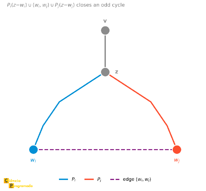
The subpath of \(P_i\) that goes from \(v\) to \(z\), denoted \(P_i(v{-}z)\), has the same length as the subpath \(P_j(v{-}z)\); otherwise, one of the two paths would not be the shortest to its respective destination (it would suffice to swap the longer stretch for the shorter stretch of the other path to obtain a shortcut). Since \(P_i\) and \(P_j\) have even length in total, and the parts from \(v\) to \(z\) have the same length, the remaining subpaths \(P_i(z{-}w_i)\) and \(P_j(z{-}w_j)\) have the same parity as each other (both even or both odd).
But the edge \((w_i, w_j)\) exists by hypothesis. Hence the route \(P_i(z{-}w_i) \cup (w_i,w_j) \cup P_j(z{-}w_j)\), which goes from \(z\) to \(w_i\), then to \(w_j\) through the edge, and back to \(z\) along \(P_j\), forms a cycle of length \(\text{len}(P_i(z{-}w_i)) + 1 + \text{len}(P_j(z{-}w_j))\). Since the two terms have the same parity, this sum is always odd (even + even + 1, or odd + odd + 1). This produces an odd cycle in \(G\), contradicting the hypothesis that \(G\) contains no odd cycle.
This contradiction shows that the edge \((w_i, w_j)\) cannot exist (and, analogously, no edge inside \(V_2\) can exist). Hence \((V_1, V_2)\) is indeed a bipartition of \(G\), that is, \(G\) is bipartite.
Therefore, with both directions, a graph is bipartite if and only if it contains no cycle of odd length, which is what we wanted to prove. \(\blacksquare\)
Every cycle \(C_n\) with \(n\) even is bipartite. Every cycle \(C_n\) with \(n\) odd is not bipartite.
Application: the proof becomes an algorithm
The construction used in the proof (\(\Leftarrow\)), which colors each vertex by the parity of its distance to a reference vertex, is the algorithm that graph libraries use to test bipartiteness. Implementing the same idea with the breadth-first search (BFS) we saw in the section on distances:
from collections import deque
import networkx as nx

def bipartition(G, source):
    """V1 = even distance from source, V2 = odd distance: the same
    construction used in the proof of the theorem."""
    color = {source: 0}
    queue = deque([source])
    while queue:
        v = queue.popleft()
        for neighbor in G.neighbors(v):
            if neighbor not in color:
                color[neighbor] = 1 - color[v]
                queue.append(neighbor)
            elif color[neighbor] == color[v]:
                return None  # edge inside the same side: not bipartite
    V1 = sorted(v for v, c in color.items() if c == 0)
    V2 = sorted(v for v, c in color.items() if c == 1)
    return V1, V2

print("C6:", bipartition(nx.cycle_graph(6), 0))
print("C5:", bipartition(nx.cycle_graph(5), 0))
C6: ([0, 2, 4], [1, 3, 5])
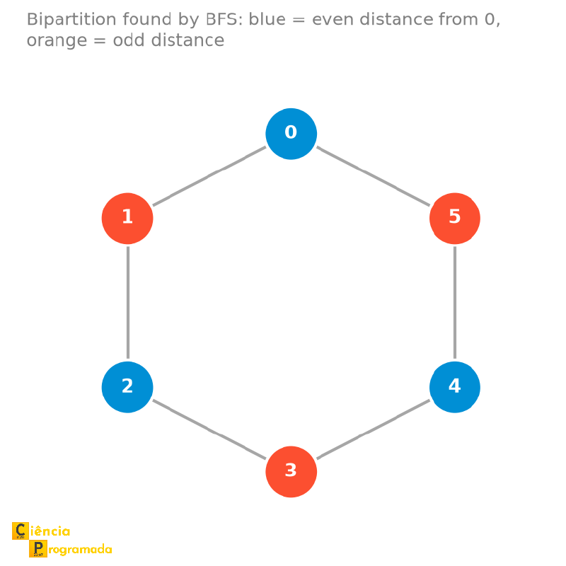
C5: NoneFor \(C_6\) (an even cycle), the function returns exactly the expected
alternating bipartition: even-position vertices on one side, odd on the
other, as the figure below shows. For \(C_5\) (an odd cycle), BFS
eventually finds an edge between two vertices of the same color (the same
contradiction exploited in the proof), and the function returns None,
confirming that no bipartition exists.
The networkx library already ships this check ready-made as
nx.is_bipartite, which agrees with our implementation:
import networkx as nx

print(nx.is_bipartite(nx.cycle_graph(6)))  # True
print(nx.is_bipartite(nx.cycle_graph(5)))  # False
Application: revisiting Zachary’s Karate Club
Zachary’s Karate Club graph, the 34-member social network that we already saw when studying vertex degree, is a good test of this article’s properties on a real graph, much larger than the examples we solved by hand:
import networkx as nx

G = nx.karate_club_graph()

print("Connected:", nx.is_connected(G))
print("Diameter:", nx.diameter(G))
print("Center:", nx.center(G))
print("Bipartite:", nx.is_bipartite(G))
Connected: True
Diameter: 5
Center: [0, 1, 2, 3, 8, 13, 19, 31]
Bipartite: FalseThe whole club is a single connected component (\(\omega(G)=1\)), with diameter 5, a little larger than that of the graph \(G\) in this article, but still small for a real social network. Note that vertex \(33\) (the club administrator, of highest degree, with \(17\) connections, as we saw in the article on degree) is not in the center: its eccentricity is \(4\), versus \(3\) for vertex \(0\). Having more connections does not guarantee being more “in the middle” of the network in terms of distance: these are different notions of centrality.
And the graph is not bipartite: a real friendship network has groups that form triangles (\(A\) and \(B\) are friends, \(B\) and \(C\) are friends, and \(A\) and \(C\) end up becoming friends too), and every triangle is an odd cycle, which is enough, by the characterization theorem, to rule out any chance of a bipartition.
Exercises #
The following exercises apply the concepts of walk, trail, path, and bipartition seen in this article, in increasing order of difficulty.
Exercise 1: Classifying sequences
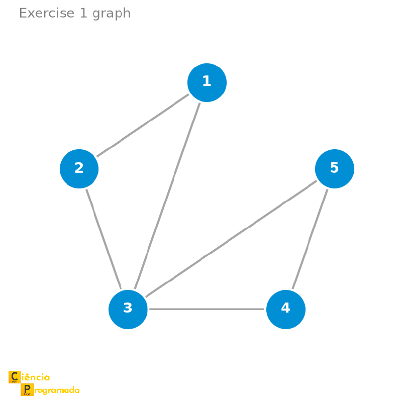
Statement: Classify each sequence below as a walk, trail, path, or none of these, in a graph with vertices \(\{1,2,3,4,5\}\) and edges \(\{1,2\}, \{2,3\}, \{3,4\}, \{4,5\}, \{1,3\}, \{3,5\}\):
(a) \(1, 2, 3, 4, 5, 3, 1\) (b) \(1, 3, 2, 4\) (c) \(1, 2, 3, 5, 4\) (d) \(1, 3, 5, 4, 3, 2\)
Solution
(a) It is a (closed) trail, because the sequence traverses all 6 edges of
the graph, each exactly once: \(\{1,2\}, \{2,3\}, \{3,4\},
\{4,5\}, \{3,5\}, \{1,3\}\). Since no edge repeats, it is a
trail, and since \(v_0 = v_6 = 1\), it is closed. It is neither a path nor a
cycle, since vertex 3 is visited twice (at positions 3 and 6).
(b) It is not valid: there is no edge \(\{2,4\}\).
(c) It is a path, because no vertex repeats and all the edges exist: \(\{1,2\}, \{2,3\}, \{3,5\}, \{5,4\}\). ✓
(d) It is a trail: no edge repeats, but vertex 3 appears twice.
The graph used in the exercise, to visualize the sequences above:
Exercise 2: Bipartite?
Statement: Determine whether the cycle \(C_6\) is bipartite and, if it is, give the bipartition.
Solution
\(C_6\) has even length, so it is bipartite by the characterization theorem. For \(C_6 = v_1-v_2-v_3-v_4-v_5-v_6-v_1\), the bipartition is \(V_1 = \{v_1, v_3, v_5\}\) and \(V_2 = \{v_2, v_4, v_6\}\). \(\blacksquare\)
Summary #
| Concept | Description |
|---|---|
| Walk | Sequence of vertices \(v_0, \ldots, v_k\) with \((v_i,v_{i+1}) \in E\); repetitions allowed |
| Trail | Walk with no repeated edges |
| Path | Walk with no repeated vertices |
| Closed trail | Closed walk (\(v_0=v_k\)) with no repeated edges |
| Cycle | Closed walk with no repeated internal vertices |
| Even / odd cycle | Cycle with an even / odd number of edges |
| Connected vertices | A path exists between them |
| Connected | Every pair of vertices is connected |
| Connected component | Connected, maximal induced subgraph (partition of \(V\)) |
| Distance \(d(v,w)\) | Length of the shortest path; \(\infty\) if \(v,w\) are disconnected |
| Breadth-first search (BFS) | Computes distances from a source in \(O(n+m)\) |
| Dijkstra’s algorithm | Distances in graphs with nonnegative weights, with a priority queue |
| Eccentricity \(e(v)\) | Greatest distance from \(v\) to any other vertex |
| Diameter | Greatest eccentricity of the graph (assumes \(G\) connected) |
| Center \(c(G)\) | Vertices of smallest eccentricity |
| Trivial / null graph | \(K_1\) (one vertex, no edges) / \(N_n\) (\(n\) vertices, no edges) |
| Bipartite | \(V = V_1 \cup V_2\), \(V_1 \cap V_2 = \emptyset\), edges only between \(V_1\) and \(V_2\) |
| Bipartite ↔ | No cycles of odd length |
Next Steps #
We have answered the opening question: we now know how to recognize whether two points of a graph are connected, measure the shortest distance between them, and decide whether the whole structure is bipartite. But walks, cycles, and connectivity do not answer this question: what is the smallest number of edges capable of keeping a graph connected, with no leftover cycle? That is the question that motivates trees, the topic of the next article in the series.


