

In 1873, the Dutch physicist Johannes Diderik van der Waals defended a doctoral thesis that solved a nagging problem: the ideal gas law, \(PV=nRT\), simply did not describe real gases near condensation, nor did it explain why, under enough pressure and temperature, a gas becomes a liquid. Van der Waals proposed a correction with two extra terms: one for the volume the molecules themselves occupy, another for the attraction between them. The resulting equation did something the ideal gas law never could: it predicted the existence of a critical point, the temperature above which liquid and vapor stop being distinct phases. The discovery earned van der Waals the Nobel Prize in Physics in 1910.
The price of the correction: the elegant linear equation \(PV=nRT\) becomes a cubic in \(V\),
$$ \left(P + \frac{an^2}{V^2}\right)(V - nb) = nRT $$But cubics, in practice, have no useful closed-form solution. And this is just one of the equations like this outside physics: from analytical chemistry to pipe engineering, the same kind of problem shows up in different disguises.
Before coming back to van der Waals, though, let’s start with a warm-up: a quadratic equation, which everyone knows how to solve, and where the interesting question is “when is it worth it”, not “how to solve it”. Then comes the cubic from the hook, and finally an equation that is not a polynomial at all.
Why Does This Matter in Chemistry and Engineering? #
- Chemical engineering: equations of state for real gases (such as van der Waals) are the basis of any industrial process design that involves compressing, liquefying or storing gases.
- Analytical chemistry: calculating the real pH of a solution (without the simplifying classroom shortcuts) matters whenever the dilution is high or the required precision is greater than that of a textbook exercise.
- Civil and mechanical engineering: sizing any pipe (water, oil, gas)
depends on the friction factor, which for decades required manual
iteration or reading a chart before
scipy.optimizeexisted. - Process industries in general: the three equations in this article show up, in the most varied forms, in any commercial chemical process simulation software.
The methods used here, brentq for root finding and numpy.roots for
polynomials, are the same ones presented in Solving Equations Numerically with SciPy,
the first article of this block. As in the previous article, on physics,
here they solve complete chemistry and engineering problems, with real
numbers.
1. Weak Acid pH: When the Classroom Shortcut Is Enough #
Every general chemistry course teaches the same recipe for calculating the pH of a weak acid. The dissociation equilibrium,
$$ HA \rightleftharpoons H^+ + A^-, \qquad K_a = \frac{x^2}{C_0 - x} $$becomes a quadratic equation in \(x = [H^+]\). The classroom recipe assumes that the dissociation is small (\(C_0 - x \approx C_0\)) and goes straight to \(x \approx \sqrt{K_a C_0}\), without solving any quadratic. It is fast and works for most exercises. But it is an approximation, and it is worth seeing how far it strays from the exact answer.
Example 1: acetic acid, exact vs. approximate
Problem statement: A solution of acetic acid (\(K_a = 1.8 \times 10^{-5}\), at 25 °C) has initial concentration \(C_0 = 0.10\) mol/L. What is the exact pH, solving the full quadratic, and what is the pH from the general chemistry approximation?
Solution:
import numpy as np
from scipy import optimize

Ka = 1.8e-5  # acetic acid
C0 = 0.10  # mol/L

# x^2 + Ka*x - Ka*C0 = 0
roots_acid = np.roots([1, Ka, -Ka * C0])
# only real, positive roots: [H+] cannot be negative or complex
x_exact = roots_acid[np.isreal(roots_acid) & (roots_acid.real > 0)].real.max()
x_approx = np.sqrt(Ka * C0)

pH_exact = -np.log10(x_exact)
pH_approx = -np.log10(x_approx)
print(f"[H+] exact: {x_exact:.6e} mol/L -> pH = {pH_exact:.4f}")
print(f"[H+] approximate: {x_approx:.6e} mol/L -> pH = {pH_approx:.4f}")
print(f"pH difference: {abs(pH_exact - pH_approx):.5f}")
[H+] exact: 1.332671e-03 mol/L -> pH = 2.8753
[H+] approximate: 1.341641e-03 mol/L -> pH = 2.8724
pH difference: 0.00291For this concentration, the difference is tiny: less than \(0.003\) pH unit, irrelevant in practice. The plot below shows why: the curve is the full quadratic, \(g(x) = x^2 + K_a x - K_a C_0\), with the exact root marked where it crosses zero. The approximation does not solve this same equation: it is the root of a simpler equation, so it does not land exactly on the curve, but it is visibly close.
import matplotlib.pyplot as plt
import numpy as np

Ka = 1.8e-5  # acetic acid
C0 = 0.10  # mol/L

roots_acid = np.roots([1, Ka, -Ka * C0])
x_exact = roots_acid[np.isreal(roots_acid) & (roots_acid.real > 0)].real.max()
x_approx = np.sqrt(Ka * C0)

x_range = np.linspace(0, x_exact * 1.5, 400)


def ph_residual(x, Ka, C0):
    return x**2 + Ka * x - Ka * C0


fig, ax = plt.subplots(figsize=(8, 5))
ax.plot(x_range * 1e3, ph_residual(x_range, Ka, C0), color="C0")
ax.axhline(0, color="gray", linewidth=1, zorder=0)
ax.scatter([x_exact * 1e3], [0], color="C2", zorder=3,
           label=f"exact root: {x_exact * 1e3:.3f} mmol/L")
ax.axvline(x_approx * 1e3, color="C1", linestyle="--",
           label=f"approximation: {x_approx * 1e3:.3f} mmol/L")
ax.legend()
ax.set_xlabel("[H+] (mmol/L)")
ax.set_ylabel("residual")
ax.set_title("Weak acid pH: exact root vs. general chemistry approximation")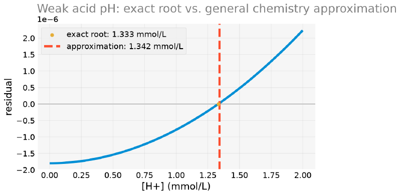
When Does the Approximation Stop Holding? #
The approximation \(C_0 - x \approx C_0\) is only good when the dissociation is small compared to \(C_0\), which fails precisely in very dilute solutions, where a larger fraction of the acid dissociates. By sweeping several concentrations on a logarithmic scale (natural in chemistry, where concentrations vary by orders of magnitude) and comparing exact and approximate pH, it becomes visible where the classroom rule of thumb stops being reliable.
import matplotlib.pyplot as plt
import numpy as np

Ka = 1.8e-5  # acetic acid

C0_range = np.logspace(-6, 0, 200)  # 1 µmol/L to 1 mol/L
pH_exact_range = []
pH_approx_range = []

for C0_i in C0_range:
    roots_i = np.roots([1, Ka, -Ka * C0_i])
    x_exact_i = roots_i[np.isreal(roots_i) & (roots_i.real > 0)].real.max()
    x_approx_i = np.sqrt(Ka * C0_i)
    pH_exact_range.append(-np.log10(x_exact_i))
    pH_approx_range.append(-np.log10(x_approx_i))

error_pH = np.abs(np.array(pH_exact_range) - np.array(pH_approx_range))

fig, ax = plt.subplots(figsize=(8, 5))
ax.semilogx(C0_range, error_pH, color="C0")
ax.axhline(0.05, color="C1", linestyle="--", label="0.05 pH unit error")
ax.set_xlabel(r"$C_0$ (mol/L)")
ax.set_ylabel("|exact pH − approximate pH|")
ax.set_title("Where the general chemistry approximation breaks down")
ax.legend()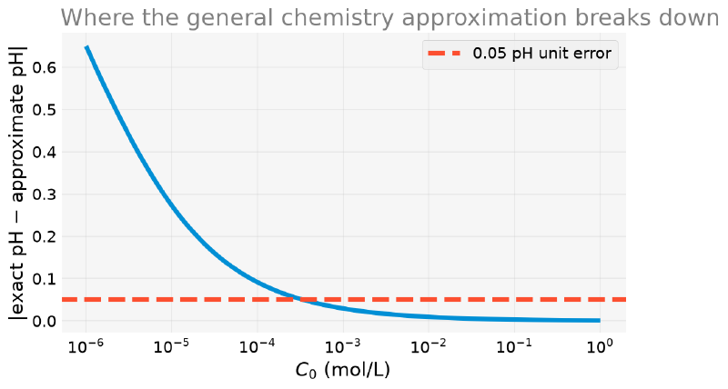
Below approximately \(3 \times 10^{-4}\) mol/L, the error already exceeds \(0.05\) pH unit and keeps growing. This is exactly the range of very dilute solutions (common in environmental and trace analyses), where the classroom recipe stops being reliable and the full quadratic becomes worth it.
This article has been calling the solution of the quadratic “exact”, as opposed to the classroom shortcut. It is exact within its own model, and that model ignores one thing: the autoprotolysis of water, \(2H_2O \rightleftharpoons H_3O^+ + OH^-\), which also produces \(H^+\).
The complete model combines the acid equilibrium, the water equilibrium (\(K_w = 10^{-14}\)), the mass balance and the charge balance \([H^+] = [A^-] + [OH^-]\). The result is a cubic:
$$[H^+]^3 + K_a[H^+]^2 - (K_aC_0 + K_w)[H^+] - K_aK_w = 0$$import numpy as np
Ka = 1.8e-5 # acetic acid
Kw = 1e-14
for C0_i in (1e-1, 1e-4, 1e-6, 1e-7):
x_quad = np.roots([1, Ka, -Ka * C0_i]).max()
r = np.roots([1, Ka, -(Ka * C0_i + Kw), -Ka * Kw])
x_full = max(r[np.abs(r.imag) < 1e-12].real)
print(f"C0={C0_i:.0e}: pH quadratic={-np.log10(x_quad):.4f}"
f" pH with water={-np.log10(x_full):.4f}")C0=1e-01: pH quadratic=2.8753 pH with water=2.8753
C0=1e-04: pH quadratic=4.4638 pH with water=4.4638
C0=1e-06: pH quadratic=6.0223 pH with water=6.0178
C0=1e-07: pH quadratic=7.0024 pH with water=6.7927For acetic acid at \(0.10\) mol/L, nothing changes: water is irrelevant there. But look at the last case, \(C_0 = 10^{-7}\) mol/L: the quadratic returns pH \(7.0024\), that is, it predicts that an acid solution is slightly basic. This is a physical absurdity, and it comes precisely from ignoring water, which, at this dilution, contributes more \(H^+\) than the acid itself. The complete model gives \(6.79\), correctly acidic.
The lesson holds for the whole article, and is the reason this callout exists: “exact” is always exact relative to a model. Going down one step of approximation (from the shortcut to the quadratic) solves one problem and reveals the next. The plot above measures the distance between step 1 and step 2; below \(10^{-6}\) mol/L, step 3 would be needed.
2. Van der Waals: Back to the Hook #
Back to the equation that opened this article. The molar volume of a real
gas has no closed-form solution, but brentq solves it without difficulty,
as long as the bracket contains the right physical root.
Example 2: real CO2 vs. ideal CO2
Problem statement: One mole of CO2 is at \(P = 10\) atm and \(T = 300\) K. What is the molar volume from the ideal gas law, and what is the real volume from the van der Waals equation (\(a = 3.640\) L²·atm/mol², \(b = 0.04267\) L/mol)?
Solution:
from scipy import optimize

R = 0.082057366080960  # atm L / (mol K)
a_co2, b_co2 = 3.640, 0.04267  # L^2 atm / mol^2 ; L / mol
P_val, T_val, n_val = 10.0, 300.0, 1.0


def van_der_waals(V):
    return (P_val + a_co2 * n_val**2 / V**2) * (V - n_val * b_co2) - n_val * R * T_val


V_ideal = n_val * R * T_val / P_val
V_vdw = optimize.brentq(van_der_waals, 0.01, 10)
print("V ideal:", V_ideal, "L")
print("V van der Waals:", V_vdw, "L")
print("deviation:", (V_vdw - V_ideal) / V_ideal * 100, "%")
V ideal: 2.4617209824287998 L
V van der Waals: 2.3524663349745696 L
deviation: -4.438140968617679 %Real CO2 occupies about 4.4% less volume than the ideal gas would
predict: under these conditions, the attraction between molecules (the term
\(a\)) slightly outweighs the effect of their own volume (the term
\(b\)). The plot below shows both solutions: the dashed line is the ideal
volume, the dot is the real root found by brentq.
import matplotlib.pyplot as plt
import numpy as np
from scipy import optimize

R = 0.082057366080960  # atm L / (mol K)
a_co2, b_co2 = 3.640, 0.04267  # L^2 atm / mol^2 ; L / mol
P_val, T_val, n_val = 10.0, 300.0, 1.0


def van_der_waals(V):
    return (P_val + a_co2 * n_val**2 / V**2) * (V - n_val * b_co2) - n_val * R * T_val


V_ideal = n_val * R * T_val / P_val
V_vdw = optimize.brentq(van_der_waals, 0.01, 10)

V_range = np.linspace(0.05, 3, 500)
fig, ax = plt.subplots(figsize=(8, 5))
ax.plot(V_range, van_der_waals(V_range), color="C0")
ax.axhline(0, color="gray", linewidth=1, zorder=0)
ax.axvline(V_ideal, color="C1", linestyle="--", label="ideal V")
ax.scatter([V_vdw], [0], color="C2", zorder=3, label="van der Waals V")
ax.legend()
ax.set_xlabel("V (L)")
ax.set_ylabel("van der Waals residual")
ax.set_title("Ideal gas vs. real gas (CO₂)")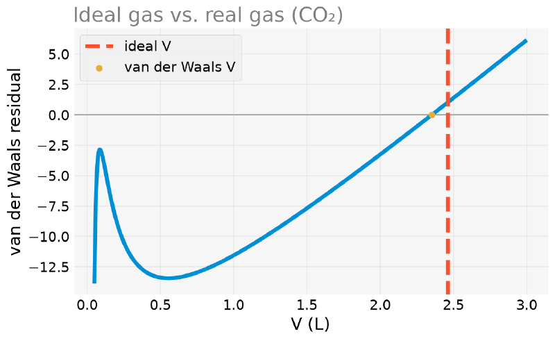
What If the Cubic Has More Than One Real Root? #
brentq only finds the root you already expected
In Example 2, brentq silently assumed that there was only one physical
root in the bracket (0.01, 10). But the van der Waals equation is a real
cubic in \(V\), and cubics can have up to 3 real roots. brentq never
warns that other roots exist outside the given bracket; it simply returns
the first one it finds inside it.
To find all of them at once, we first need to recognize the cubic hidden in the usual form of the equation. The trick is to multiply everything by \(V^2\) and expand:
$$ \left(P + \frac{an^2}{V^2}\right)(V - nb) = nRT $$$$ PV - Pnb + \frac{an^2}{V} - \frac{an^3b}{V^2} = nRT $$Multiplying by \(V^2\) and grouping by power of \(V\):
$$ PV^3 - (Pnb + nRT)V^2 + an^2V - an^3b = 0 $$Now it is a degree 3 polynomial with explicit coefficients: exactly the
format that numpy.roots expects.
Three real roots appear below the critical temperature \(T_c\), exactly the region
of the P-V diagram where liquid and vapor coexist: the “loop” in the phase
diagrams of real gases, and the same discovery that earned van der Waals
the Nobel. To find all the roots at once, we rewrite the equation in the
explicit polynomial form,
\(PV^3 - (Pnb+nRT)V^2 + an^2V - an^3b = 0\), and use once again the same
numpy.roots from the previous section, the tool that the
next article in this series
will explore in depth.
Instead of choosing \(T\) and \(P\) arbitrarily until the cubic yields 3 roots, we use the law of corresponding states:
Defining the reduced temperature and pressure \(T_r = T/T_c\) and \(P_r = P/P_c\) (relative to the critical values \(T_c\) and \(P_c\) of the substance), any fluid described by the van der Waals equation with \(T_r < 1\) has a range of pressures where the cubic admits 3 real roots, regardless of the substance. This is what gives the law its practical usefulness.
The caveat matters: this is a property of the equation, not a fact about real gases. Real gases only obey the law of corresponding states approximately, and van der Waals itself is a rather crude equation of state near the critical point; this is why Redlich-Kwong, Soave and Peng-Robinson exist, all more accurate and all still cubic in \(V\), that is, solved in exactly the same way.
import numpy as np

R = 0.082057366080960  # atm L / (mol K)
a_co2, b_co2 = 3.640, 0.04267  # L^2 atm / mol^2 ; L / mol

T_c = 8 * a_co2 / (27 * R * b_co2)
P_c = a_co2 / (27 * b_co2**2)
print(f"CO2: T_c = {T_c:.1f} K, P_c = {P_c:.1f} atm")


def van_der_waals_coeffs(P, T, n=1.0):
    c3 = P
    c2 = -(P * n * b_co2 + n * R * T)
    c1 = a_co2 * n**2
    c0 = -a_co2 * n**3 * b_co2
    return [c3, c2, c1, c0]


T_r, P_r = 0.84, 0.41
T_subcritical = T_r * T_c
P_subcritical = P_r * P_c
print(f"T_r = {T_r} -> T = {T_subcritical:.1f} K")
print(f"P_r = {P_r} -> P = {P_subcritical:.1f} atm")

roots = np.roots(van_der_waals_coeffs(P_subcritical, T_subcritical))
print("roots (may include complex ones):", roots)

positive_real_roots = np.sort(roots[(np.abs(roots.imag) < 1e-8) & (roots.real > 0)].real)
print("positive real roots, sorted:", positive_real_roots)
CO2: T_c = 308.0 K, P_c = 74.0 atm
T_r = 0.84 -> T = 258.7 K
P_r = 0.41 -> P = 30.4 atm
roots (may include complex ones): [0.53623521 0.13527776 0.07052874]
positive real roots, sorted: [0.07052874 0.13527776 0.53623521]Three positive real roots. Physically:
- the smallest, \(V \approx 0.0705\) L/mol, is the molar volume of the liquid (near the covolume \(b\), molecules tightly packed);
- the largest, \(V \approx 0.5362\) L/mol, is the molar volume of the vapor;
- the middle one, \(V \approx 0.1353\) L/mol, does not correspond to any stable physical state: it is the part of the curve where \(\partial P/\partial V > 0\), thermodynamically unstable.
Saying that the three roots mark the region where liquid and vapor coexist is a convenient simplification, but it is not quite right. Having three real roots means being inside the van der Waals loop, and the loop is wider than the true coexistence.
Equilibrium coexistence only happens at one specific pressure for each temperature: the saturation pressure, the one at which liquid and vapor have the same chemical potential. It is determined by the Maxwell equal-area construction: draw the horizontal line that cuts the loop so that the two enclosed areas above and below it are equal.
Away from that specific pressure, the three roots still exist, but what they describe is something else: one of the phases is stable and the other is metastable, that is, superheated liquid or supercooled vapor, states that do exist (it is what lets you superheat water in the microwave), but that collapse at the slightest disturbance. The middle root, on the other hand, describes no state under any condition.
For this article, this changes nothing: the three roots are the same, and the point (that mathematics hands over options and physics chooses) still stands. But it is worth knowing that the label “coexistence” hides one extra geometric construction.
numpy.roots knows nothing about thermodynamics: it only returns the 3
mathematical roots of the cubic. Physics, thermodynamic stability, is what
decides which of them is the “true” volume in each phase. It is the same
kind of care we saw in the article on
polynomials with SymPy
(Poly.all_roots() vs. Poly.real_roots()), only now with a concrete
physical meaning behind each root. The plot below marks the three roots on
the curve, annotating the physical role of each one.
import matplotlib.pyplot as plt
import numpy as np

R = 0.082057366080960  # atm L / (mol K)
a_co2, b_co2 = 3.640, 0.04267  # L^2 atm / mol^2 ; L / mol
T_c = 8 * a_co2 / (27 * R * b_co2)
P_c = a_co2 / (27 * b_co2**2)
T_subcritical = 0.84 * T_c
P_subcritical = 0.41 * P_c


def van_der_waals_coeffs(P, T, n=1.0):
    c3 = P
    c2 = -(P * n * b_co2 + n * R * T)
    c1 = a_co2 * n**2
    c0 = -a_co2 * n**3 * b_co2
    return [c3, c2, c1, c0]


roots = np.roots(van_der_waals_coeffs(P_subcritical, T_subcritical))
positive_real_roots = np.sort(roots[(np.abs(roots.imag) < 1e-8) & (roots.real > 0)].real)

V_range_sub = np.linspace(0.05, 1.5, 800)


def van_der_waals_sub(V):
    return (P_subcritical + a_co2 / V**2) * (V - b_co2) - R * T_subcritical


V_liquid, V_unstable, V_vapor = positive_real_roots

fig, ax = plt.subplots(figsize=(8, 5))
ax.plot(V_range_sub, van_der_waals_sub(V_range_sub), color="C0")
ax.axhline(0, color="gray", linewidth=1, zorder=0)
ax.scatter([V_liquid, V_unstable, V_vapor], [0, 0, 0], color="C2", zorder=3,
           label="3 real roots")
ax.annotate("liquid", (V_liquid, 0), textcoords="offset points", xytext=(-55, 45),
            ha="left", arrowprops=dict(arrowstyle="-", color="gray", linewidth=1))
ax.annotate("unstable", (V_unstable, 0), textcoords="offset points", xytext=(40, 55),
            ha="center", arrowprops=dict(arrowstyle="-", color="gray", linewidth=1))
ax.annotate("vapor", (V_vapor, 0), textcoords="offset points", xytext=(0, 12), ha="center")
ax.legend()
ax.set_xlabel("V (L/mol)")
ax.set_ylabel("van der Waals residual")
ax.set_title(f"Van der Waals below T_c: 3 real roots (T={T_subcritical:.0f} K)")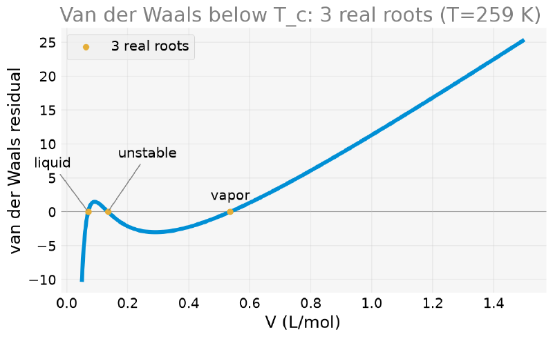
The Isotherms, and What “Coexistence” Really Requires #
All the figures in this section showed the residual \(f(V)\), perfect for seeing “this is a root problem”, but silent about the physics. The canonical figure for the subject is the \(P\)-\(V\) diagram with isotherms, and it is worth drawing it, because in it the caveat from the previous callout stops being abstract.
Finding the saturation pressure is itself a root problem, only a nested one. Maxwell’s condition is that the horizontal line divides the loop into equal areas:
$$ \int_{V_{liq}}^{V_{vap}} \left[P_{vdW}(V) - P_{sat}\right] dV = 0 $$And it has an elementary antiderivative, \(\int P dV = RT\ln(V-b) + a/V\), which avoids numerical quadrature near the singularity at \(V = b\):
import numpy as np
from scipy import optimize

R = 0.082057366080960  # atm L / (mol K)
a_co2, b_co2 = 3.640, 0.04267  # L^2 atm / mol^2 ; L / mol
T_c = 8 * a_co2 / (27 * R * b_co2)
P_c = a_co2 / (27 * b_co2**2)
T_subcritical = 0.84 * T_c
P_subcritical = 0.41 * P_c


def van_der_waals_coeffs(P, T, n=1.0):
    c3 = P
    c2 = -(P * n * b_co2 + n * R * T)
    c1 = a_co2 * n**2
    c0 = -a_co2 * n**3 * b_co2
    return [c3, c2, c1, c0]


def P_vdw(V, T):
    return R * T / (V - b_co2) - a_co2 / V**2


def dPdV_vdw(V, T):
    return -R * T / (V - b_co2) ** 2 + 2 * a_co2 / V**3


def spinodals(T):
    """The two V where dP/dV = 0: the bottom of the valley and the top of the loop's hump."""
    return (optimize.brentq(dPdV_vdw, b_co2 * 1.001, 3 * b_co2, args=(T,)),
            optimize.brentq(dPdV_vdw, 3 * b_co2, 50, args=(T,)))


def saturation_pressure(T):
    V_min, V_max = spinodals(T)                     # where dP/dV = 0
    P_lo, P_hi = P_vdw(V_min, T), P_vdw(V_max, T)   # local minimum and maximum of the loop

    def antiderivative(V):
        return R * T * np.log(V - b_co2) + a_co2 / V

    def imbalance(P):
        r = np.roots(van_der_waals_coeffs(P, T))
        r = np.sort(r[np.abs(r.imag) < 1e-9].real)
        return (antiderivative(r[-1]) - antiderivative(r[0])) - P * (r[-1] - r[0])

    return optimize.brentq(imbalance, max(P_lo, 1e-9) * 1.0001, P_hi * 0.9999)


P_sat = saturation_pressure(T_subcritical)
print(f"P_sat = {P_sat:.2f} atm  ->  Pr = {P_sat / P_c:.3f}")
P_sat = 35.44 atm -> Pr = 0.479The example used \(P_r = 0.41\), but the equilibrium pressure at that temperature is \(P_r = 0.479\). The three roots exist at both pressures, but only at one of them do liquid and vapor truly coexist. At the other, one of the phases is metastable.
The van der Waals saturation curve in reduced variables is tabulated, and does not depend on the substance. It serves as a test for the code:
| \(T_r\) | \(P_r\) computed | \(P_r\) tabulated |
|---|---|---|
| 0.95 | 0.8119 | 0.812 |
| 0.90 | 0.6470 | 0.647 |
| 0.85 | 0.5045 | 0.504 |
| 0.80 | 0.3834 | 0.383 |
It matches in all four. A word of warning: a brentq that receives a
bracket with inverted endpoints does not complain and returns a plausible
number (here, \(P_r = 0.725\) for \(T_r = 0.90\)). Only the comparison
with the table gives the error away.
The figure below shows, on the left, the classic isotherms (above, at and below \(T_c\)) with the critical point marked; and on the right, a zoom into the subcritical loop with the Maxwell construction drawn:
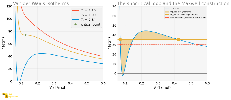
In the right panel, the two shaded regions have very different shapes (the left one is tall and narrow, the right one is low and wide), but the same area. This equality is what defines \(P_{sat}\): the equilibrium horizontal is the only height at which the two compensate each other.
Also notice where the bottom of the loop ends up: below zero, down to about \(-2\) atm. Van der Waals predicts negative pressure in that range, which describes no real equilibrium state; it is one more sign that the central stretch of the loop is not physics: it is the price of forcing a single smooth equation across a region where, in fact, two phases coexist. The Maxwell construction exists precisely to replace that stretch with the horizontal line.
Notice the left panel as well: above \(T_c\) the isotherm descends with no undulation at all. There is no loop, no three roots, no phase transition. This is exactly what van der Waals predicted and what the ideal gas law could never predict: there is a temperature above which liquid and vapor stop being distinct things.
3. Colebrook Friction Factor: From the Slide Rule to brentq
#
Last equation, and the newest of the three, but the one that shows up most in the day-to-day of an engineering project. Published by Cyril Colebrook in 1939, based on experiments he did with Cedric White in 1937 (which is why it is also called the Colebrook-White equation), it gives the friction factor in turbulent flow inside pipes in an implicit form (see the entry Darcy friction factor formulae):
$$ \frac{1}{\sqrt{f}} = -2\log_{10}\left(\frac{\varepsilon/D}{3.7} + \frac{2.51}{Re\sqrt{f}}\right) $$\(f\) appears on both sides, and inside a logarithm: there is no way to
isolate it. Five years later, in 1944, Lewis Moody published the chart that
would carry his name precisely to spare engineers this calculation: with a
ruler and an eye, one read \(f\) off a plot instead of iterating by hand.
That is how it went, for decades, until programmable calculators. Today, it
is a call to brentq, and, later in this section, we rebuild Moody’s chart
itself from it.
Example 3: water in a commercial steel pipe
Problem statement: Water flows at \(2\) m/s (typical design velocity) in a commercial steel pipe with a diameter of \(100\) mm. The absolute roughness of commercial steel is \(\varepsilon \approx 0.045\) mm (a tabulated engineering value); the kinematic viscosity of water at 20 °C is \(\nu \approx 10^{-6}\) m²/s. What is the friction factor?
Solution:
import numpy as np
from scipy import optimize

D_pipe = 0.10  # m — 100 mm pipe
eps_steel = 0.045e-3  # m — absolute roughness of commercial steel (tabulated)
eps_over_D = eps_steel / D_pipe

nu_water = 1.0e-6  # m²/s — kinematic viscosity of water at ~20°C
v_flow = 2.0  # m/s — typical design velocity in pipes
Re = v_flow * D_pipe / nu_water

print(f"eps/D = {eps_over_D}")
print(f"Re = {Re:.0f}")


def colebrook(f, eps_D, Re_):
    return 1 / np.sqrt(f) + 2 * np.log10(eps_D / 3.7 + 2.51 / (Re_ * np.sqrt(f)))


f_friction = optimize.brentq(colebrook, 1e-4, 0.5, args=(eps_over_D, Re))
print("friction factor (brentq):", f_friction)
eps/D = 0.00045
Re = 200000
friction factor (brentq): 0.01856015225418919As in the previous examples, it is worth seeing the curve of the Colebrook equation (rearranged as a residual) crossing zero at the friction factor found.
import matplotlib.pyplot as plt
import numpy as np
from scipy import optimize

D_pipe = 0.10  # m — 100 mm pipe
eps_steel = 0.045e-3  # m — absolute roughness of commercial steel (tabulated)
eps_over_D = eps_steel / D_pipe

nu_water = 1.0e-6  # m²/s — kinematic viscosity of water at ~20°C
v_flow = 2.0  # m/s — typical design velocity in pipes
Re = v_flow * D_pipe / nu_water


def colebrook(f, eps_D, Re_):
    return 1 / np.sqrt(f) + 2 * np.log10(eps_D / 3.7 + 2.51 / (Re_ * np.sqrt(f)))


f_friction = optimize.brentq(colebrook, 1e-4, 0.5, args=(eps_over_D, Re))

f_range = np.linspace(0.008, 0.1, 400)
fig, ax = plt.subplots(figsize=(8, 5))
ax.plot(f_range, colebrook(f_range, eps_over_D, Re), color="C0")
ax.axhline(0, color="gray", linewidth=1, zorder=0)
ax.scatter([f_friction], [0], color="C2", zorder=3, label=f"f ≈ {f_friction:.4f}")
ax.legend()
ax.set_xlabel("f")
ax.set_ylabel("Colebrook residual")
ax.set_title("Friction factor: Colebrook as a root-finding problem")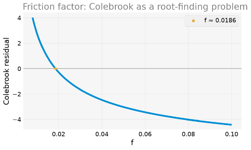
The Manual Iteration Behind the Phrase “Before Calculators” #
The Colebrook equation is implicit (\(f\) appears on both sides), but it can be rearranged by isolating \(f\) on the left-hand side:
$$ f = \left[-2\log_{10}\left(\frac{\varepsilon/D}{3.7} + \frac{2.51}{Re\sqrt{f}}\right)\right]^{-2} $$By guessing an initial value of \(f\) and repeatedly substituting from the right-hand side to the left-hand side, the fixed-point iteration, we can solve the equation with no sophisticated method at all. It is exactly what engineers did by hand, or with tables, before calculators and computers.
import numpy as np
from scipy import optimize

D_pipe = 0.10  # m — 100 mm pipe
eps_steel = 0.045e-3  # m — absolute roughness of commercial steel (tabulated)
eps_over_D = eps_steel / D_pipe

nu_water = 1.0e-6  # m²/s — kinematic viscosity of water at ~20°C
v_flow = 2.0  # m/s — typical design velocity in pipes
Re = v_flow * D_pipe / nu_water


def colebrook(f, eps_D, Re_):
    return 1 / np.sqrt(f) + 2 * np.log10(eps_D / 3.7 + 2.51 / (Re_ * np.sqrt(f)))


f_friction = optimize.brentq(colebrook, 1e-4, 0.5, args=(eps_over_D, Re))


def colebrook_fixed_point(f, eps_D, Re_):
    return (-2 * np.log10(eps_D / 3.7 + 2.51 / (Re_ * np.sqrt(f)))) ** -2


f_current = 0.02  # reasonable initial guess (typical order of magnitude)
f_history = [f_current]
for _ in range(8):
    f_current = colebrook_fixed_point(f_current, eps_over_D, Re)
    f_history.append(f_current)

for i, f_i in enumerate(f_history):
    print(f"iteration {i}: f = {f_i:.8f}   error vs. brentq = {abs(f_i - f_friction):.2e}")
iteration 0: f = 0.02000000 error vs. brentq = 1.44e-03
iteration 1: f = 0.01849038 error vs. brentq = 6.98e-05
iteration 2: f = 0.01856372 error vs. brentq = 3.57e-06
iteration 3: f = 0.01855997 error vs. brentq = 1.82e-07
iteration 4: f = 0.01856016 error vs. brentq = 9.28e-09
iteration 5: f = 0.01856015 error vs. brentq = 4.73e-10
iteration 6: f = 0.01856015 error vs. brentq = 2.41e-11
iteration 7: f = 0.01856015 error vs. brentq = 1.23e-12
iteration 8: f = 0.01856015 error vs. brentq = 6.28e-14The plot below shows this convergence on a logarithmic scale: the error drops roughly linearly with each iteration.
import matplotlib.pyplot as plt
import numpy as np
from scipy import optimize

D_pipe = 0.10  # m — 100 mm pipe
eps_steel = 0.045e-3  # m — absolute roughness of commercial steel (tabulated)
eps_over_D = eps_steel / D_pipe

nu_water = 1.0e-6  # m²/s — kinematic viscosity of water at ~20°C
v_flow = 2.0  # m/s — typical design velocity in pipes
Re = v_flow * D_pipe / nu_water


def colebrook(f, eps_D, Re_):
    return 1 / np.sqrt(f) + 2 * np.log10(eps_D / 3.7 + 2.51 / (Re_ * np.sqrt(f)))


f_friction = optimize.brentq(colebrook, 1e-4, 0.5, args=(eps_over_D, Re))


def colebrook_fixed_point(f, eps_D, Re_):
    return (-2 * np.log10(eps_D / 3.7 + 2.51 / (Re_ * np.sqrt(f)))) ** -2


f_history = [0.02]
for _ in range(8):
    f_history.append(colebrook_fixed_point(f_history[-1], eps_over_D, Re))

fig, ax = plt.subplots(figsize=(8, 5))
fixed_point_error = [abs(f_i - f_friction) for f_i in f_history]
ax.semilogy(range(len(fixed_point_error)), fixed_point_error, "o-", color="C0")
ax.set_xlabel("iteration")
ax.set_ylabel("|f − f_brentq|")
ax.set_title("Colebrook fixed-point iteration converging")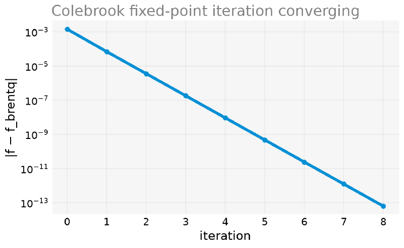
It converged to the same value as brentq in a few iterations, with no need
for a bracket or a derivative, just repeating the substitution. It is less
robust than brentq in general (fixed-point formulas can diverge depending
on how the equation is rearranged), but it shows that the “magic” behind a
call to brentq is, deep down, the same manual idea that existed decades
before.
Swamee-Jain: the Explicit Approximation the Industry Uses #
There is a third path, between manual iteration and brentq, and it
completes the arc. In 1976, Prabhata Swamee and Akalank Jain published an
explicit formula that approximates Colebrook with no iteration at all,
in a single line of computation:
import numpy as np
from scipy import optimize


def colebrook(f, eps_D, Re_):
    return 1 / np.sqrt(f) + 2 * np.log10(eps_D / 3.7 + 2.51 / (Re_ * np.sqrt(f)))


def swamee_jain(eps_D, Re_):
    return 0.25 / np.log10(eps_D / 3.7 + 5.74 / Re_**0.9) ** 2


print(f"{'Re':>8} {'eps/D':>9} {'brentq':>9} {'Swamee-Jain':>12} {'error':>7}")
for Re_i in (1e4, 2e5, 1e6, 1e7):
    for eps_i in (1e-7, 0.00045, 0.01):
        f_exact = optimize.brentq(colebrook, 1e-4, 0.5, args=(eps_i, Re_i))
        f_approx = swamee_jain(eps_i, Re_i)
        print(f"{Re_i:>8.0e} {eps_i:>9.5f} {f_exact:>9.5f} {f_approx:>12.5f}"
              f" {100*(f_approx-f_exact)/f_exact:>+6.2f}%")
Re eps/D brentq Swamee-Jain error
1e+04 0.00000 0.03088 0.03097 +0.29%
1e+04 0.00045 0.03157 0.03175 +0.58%
1e+04 0.01000 0.04313 0.04404 +2.12%
2e+05 0.00000 0.01564 0.01553 -0.68%
2e+05 0.00045 0.01856 0.01867 +0.57%
2e+05 0.01000 0.03821 0.03836 +0.40%
1e+06 0.00000 0.01165 0.01161 -0.33%
1e+06 0.00045 0.01686 0.01695 +0.56%
1e+06 0.01000 0.03796 0.03801 +0.12%
1e+07 0.00000 0.00811 0.00815 +0.50%
1e+07 0.00045 0.01637 0.01640 +0.16%
1e+07 0.01000 0.03791 0.03792 +0.02%Error below \(1\%\) over almost the entire useful range, reaching \(2\%\) only in the most extreme corner (a very rough pipe at low Reynolds number). For sizing a pipe (where the tabulated roughness already has an uncertainty larger than that), it is more than enough, and that is why Swamee-Jain appears in design spreadsheets to this day.
This closes a three-step arc that repeats throughout engineering:
| Approach | Cost | When to use |
|---|---|---|
| Implicit (Colebrook, 1939) | requires iteration | it is the reference: defines the “right” value |
| Manual iterative (fixed point) | ~5 substitutions by hand | when there is no computer |
| Approximate explicit (Swamee-Jain, 1976) | one line, no iteration | when \(1\%\) is enough, almost always, in practice |
brentq did not make the last two obsolete: it made the first one cheap
enough to be used directly. But knowing that the others exist explains why
so many engineering spreadsheets still call no solver at all.
Moody Chart #
The Colebrook equation only holds for turbulent flow
(\(Re \gtrsim 4000\)); in the laminar regime the friction factor has a
closed-form formula, \(f = 64/Re\). By solving Colebrook via brentq for a
range of Reynolds numbers and several relative roughnesses, we rebuild the
Moody chart, a classic
graphical representation that relates the friction factor, the Reynolds
number and the relative roughness, one of the classic figures of fluid
engineering.
import matplotlib.pyplot as plt
import numpy as np
from scipy import optimize

D_pipe = 0.10  # m — 100 mm pipe
eps_steel = 0.045e-3  # m — absolute roughness of commercial steel (tabulated)
eps_over_D = eps_steel / D_pipe

nu_water = 1.0e-6  # m²/s — kinematic viscosity of water at ~20°C
v_flow = 2.0  # m/s — typical design velocity in pipes
Re = v_flow * D_pipe / nu_water


def colebrook(f, eps_D, Re_):
    return 1 / np.sqrt(f) + 2 * np.log10(eps_D / 3.7 + 2.51 / (Re_ * np.sqrt(f)))


f_friction = optimize.brentq(colebrook, 1e-4, 0.5, args=(eps_over_D, Re))

Re_range = np.logspace(np.log10(4000), 8, 200)  # turbulent regime
roughnesses = [0.0, 0.00001, eps_over_D, 0.01]  # includes the steel pipe from the example

# note on the max(..., 1e-7) that appears below: "smooth pipe" is eps/D = 0, but
# then the log10 argument becomes just the Reynolds term — which is legitimate, and
# is in fact the smooth limit. The 1e-7 floor exists only so that the eps/D = 0 case
# does not produce an exact zero inside the log in any variant of the formula; it is
# a value small enough to be indistinguishable from zero in the result

fig, ax = plt.subplots(figsize=(9, 6))
for eps_D_i in roughnesses:
    f_vals = [optimize.brentq(colebrook, 1e-4, 0.5, args=(max(eps_D_i, 1e-7), Re_i))
              for Re_i in Re_range]
    if eps_D_i == 0.0:
        label = "smooth pipe (ε/D → 0)"
    elif eps_D_i == eps_over_D:
        label = f"ε/D = {eps_D_i:g} (example pipe)"
    else:
        label = f"ε/D = {eps_D_i:g}"
    ax.loglog(Re_range, f_vals, label=label)

ax.scatter([Re], [f_friction], color="black", marker="*", s=220, zorder=4,
           edgecolors="white", linewidths=1.2, label="example (Re, f)")
ax.set_xlabel("Reynolds number (Re)")
ax.set_ylabel("friction factor (f)")
ax.set_title("Moody chart (turbulent regime, via Colebrook + brentq)")
ax.legend(fontsize=10)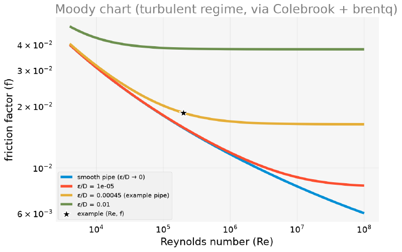
The example’s steel pipe (highlighted curve) is clearly above the smooth
pipe: the real roughness of the material noticeably increases friction even
in fully established turbulent flow. This is the kind of reading (how the
friction factor responds to Reynolds and to roughness, simultaneously) that
the Moody chart delivered before any calculator, and that brentq rebuilds
here in 800 function calls (4 curves × 200 Reynolds points each).
Summary Table #
| Problem | Equation | Method | Result |
|---|---|---|---|
| Weak acid pH | \(x^2 + K_a x - K_a C_0 = 0\) | numpy.roots |
Exact: pH \(\approx 2.875\); approximate: pH \(\approx 2.872\) (difference \(0.003\)) |
| Where the approximation fails | Same equation, variable \(C_0\) | repeated numpy.roots |
Error exceeds \(0.05\) pH unit below \(C_0 \approx 3\times10^{-4}\) mol/L |
| Molar volume of real CO2 | \((P+an^2/V^2)(V-nb)=nRT\) | brentq |
\(V \approx 2.35\) L, \(4.4\%\) smaller than the ideal volume |
| Liquid-vapor coexistence | Same cubic, \(T_r=0.84\), \(P_r=0.41\) | numpy.roots |
\(T_c \approx 308.0\) K, \(P_c \approx 74.0\) atm; 3 real roots: liquid \(\approx 0.071\), unstable \(\approx 0.135\), vapor \(\approx 0.536\) L/mol |
| Friction factor (Colebrook) | \(1/\sqrt{f} = -2\log_{10}(\ldots)\) | brentq |
\(f \approx 0.0186\) for a steel pipe, \(Re=200{,}000\) |
| Fixed-point iteration | Same equation, isolating \(f\) | Repeated substitution | Converges to the brentq value in \(\sim\)5 iterations |
| Moody chart | Colebrook for several \(Re\) and \(\varepsilon/D\) | repeated brentq (800x) |
Rebuilds the classic chart; example pipe well above the smooth pipe curve |
Next Steps: End of the Numerical Equations Arc #
This article closes the three-part arc on solving equations numerically with SciPy and NumPy. The first article presented the methods (bisection, Brent, Newton, nonlinear systems) in didactic examples; the second applied those methods to physics, from planetary orbits to projectiles with air resistance; this third one took the same methods to chemistry and engineering, always starting from a real numerical scenario, never from an arbitrary value.
What the three articles have in common is the type of problem: always a
scalar equation, or a small system, solved point by point. A whole piece is
missing: what about when the object of interest is not the root of some
equation, but a polynomial, with its own algebra of derivatives, integrals,
products and fitting to experimental data? In the next article, Polynomials with NumPy,
we see how NumPy treats polynomials as a first-class object, from the same
numpy.roots already used in this article to the task that SymPy does not do
well: fitting a curve to real noisy data.


