

Ask SymPy to integrate \(e^{-x^2}\) and it won’t complain, won’t hang,
won’t return an error. It will answer sqrt(pi)*erf(x)/2, and that answer,
however much it may look like a dodge, is the most honest thing it could
possibly say.
Because \(\int e^{-x^2}dx\) has no elementary antiderivative. There is no finite combination of polynomials, exponentials, logarithms, sines and cosines whose derivative is \(e^{-x^2}\). And this is not a limitation of SymPy, nor an open problem waiting for someone clever enough: it is a theorem, proved by Joseph Liouville in the 1830s. The antiderivative exists (every continuous function has one); it just can’t be written with the alphabet of functions you learn in high school.
What SymPy did was give it a name: erf, the error function. It is a useful
answer, but notice what happened to the original question. If someone wants
to know the value of \(\int_0^1 e^{-x^2}dx\) (a number, to put in a
report), the answer sqrt(pi)*erf(1)/2 merely pushed the problem inside a
new symbol. At some point, someone will have to compute it.
This article is about that moment.
Why Does Numerical Integration Matter? #
- Chemistry and thermodynamics: enthalpy change (\(\int C_p dT\)), expansion work (\(\int P dV\)), extent of reaction. Most thermodynamic quantities are an integral, and the \(C_p\) and \(P\) data rarely come in a form you can integrate on paper.
- Physics and engineering: center of mass, moment of inertia, work, flux through a surface, accumulated charge. These are all integrals, and almost always of functions that exist only as the result of a measurement or of another simulation.
- Probability and statistics: practically every probability is the area under a density. And the normal density, \(\propto e^{-x^2/2}\), has the same shape as the \(e^{-x^2}\) that opens this article (up to a rescaling of \(x\)), and so it has no elementary antiderivative: \(z\) tables have existed since before computers.
- Experimental data: integrating a chromatographic peak to get a concentration, a power curve to get energy consumed, a velocity to get a distance. Here there is no function at all to integrate symbolically: there is a table of numbers.
Recapping the Essentials of Symbolic Integration #
The article on integrals with SymPy
showed sympy.integrate solving indefinite and definite integrals exactly.
It is worth recalling the essentials, because the numerical approach is
defined against them:
import sympy as sp

x = sp.symbols("x")
print(sp.integrate(x**2, x))            # x**3/3
print(sp.integrate(sp.sin(x), (x, 0, sp.pi)))   # 2
When the antiderivative exists and SymPy finds it, use SymPy. An exact answer is better than any approximation, and it can still be differentiated, simplified or combined with other expressions. Numerical integration is not a more modern alternative to symbolic integration: it is what you do when the symbolic kind is not available.
And it stops being available in three quite distinct situations, which this article walks through in this order:
| Situation | Example | Why SymPy can’t solve it |
|---|---|---|
| The antiderivative does not exist in elementary terms | \(\int e^{-x^2}dx\) | Liouville’s theorem: not a software limitation |
| The antiderivative exists but is useless in practice | Long integrands, with dozens of terms | The result is an expression nobody can read, and evaluating it numerically costs more than integrating directly |
| There is no function at all | A table of measurements | There is no expression to integrate; there are only numbers |
The Integral That Won’t Close #
Let’s start with the case where the impossibility is provable. SymPy receives \(e^{-x^2}\) and answers:
import sympy as sp

x = sp.symbols("x")
antiderivative = sp.integrate(sp.exp(-(x**2)), x)
print("antiderivative:", antiderivative)

definite = sp.integrate(sp.exp(-(x**2)), (x, 0, 1))
print("from 0 to 1:", definite, "=", float(definite))
antiderivative: sqrt(pi)*erf(x)/2
from 0 to 1: sqrt(pi)*erf(1)/2 = 0.746824132812427An elementary function has an elementary antiderivative only when it satisfies a rather restrictive algebraic condition. Functions such as \(e^{-x^2}\), \(\frac{\sin x}{x}\), \(\frac{1}{\ln x}\) and \(\sqrt{1 - k^2\sin^2 x}\) provably do not satisfy it.
“Elementary,” here, is a technical term: these are the functions constructible from polynomials, exponentials and logarithms by a finite number of sums, products, quotients and compositions, which includes the trigonometric functions, since they are exponentials in disguise.
The important consequence is philosophical: when SymPy returns erf, it
has not failed. It found the right answer, and the right answer is that
this antiderivative needs a new name. It is the same move that gave
\(\sqrt{2}\) a symbol of its own when it was proved not to be a ratio of
integers.
And erf is not an arbitrary function. It is, up to a normalization,
exactly the accumulated area under the Gaussian:
The factor \(2/\sqrt{\pi}\) is there so that \(\mathrm{erf}\) tends to \(1\) as \(x \to \infty\), which makes it convenient in probability. The two plots below show the relationship between the two functions, the curve and the area it accumulates:
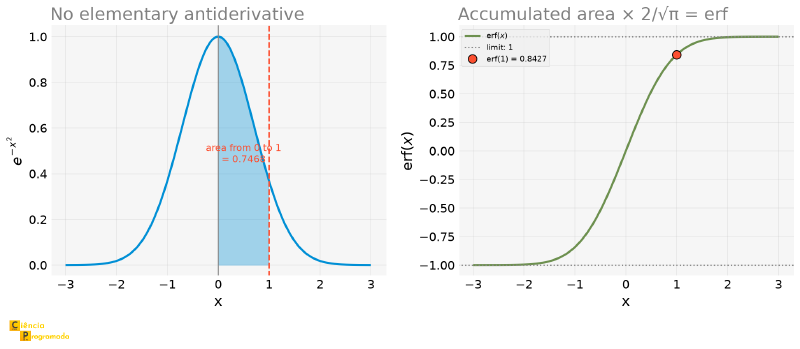
Look at the right panel. erf is a perfectly well-behaved function: smooth,
monotonic, bounded between \(-1\) and \(1\). There is nothing pathological
about it. What does not exist is a closed formula for it in elementary
terms. That is why erf lives in scipy.special, alongside dozens of other
functions that were born the same way: as a name for an integral nobody can
write any other way.
And the number we care about comes out the numerical way, directly:
import numpy as np
import sympy as sp
from scipy import integrate

x = sp.symbols("x")
definite = sp.integrate(sp.exp(-(x**2)), (x, 0, 1))

value, error = integrate.quad(lambda t: np.exp(-(t**2)), 0, 1)
print(f"quad: {value!r}")
print(f"error estimate: {error:.3e}")
print(f"difference from the symbolic value: {abs(value - float(definite)):.2e}")
quad: 0.7468241328124271
error estimate: 8.291e-15
difference from the symbolic value: 1.11e-16One line, fifteen correct digits.
quad: Integration and the Estimate of Its Own Error
#
scipy.integrate.quad is the standard tool for integrating a function of one
variable. It implements adaptive quadrature: the
QUADPACK library, written in
Fortran in the early 1980s, which SciPy’s quad uses under the hood.
“Quadrature” is the classical name for numerical integration; it comes from the Greek problem of constructing a square with the same area as a given figure.
Adaptive is the interesting part. Instead of slicing the interval into equal pieces, the method estimates the error in each piece and subdivides only where the error is large. A stretch where the function is almost a straight line is solved with few evaluations; a stretch where it oscillates is subdivided until the error estimate falls below the tolerance.
It is the same idea as the adaptive step that solve_ivp uses in
differential equations: spend effort where the problem is hard, not where
it is easy.
What sets quad apart from adding up rectangles by hand is the second
return value: an estimate of its own error. Few numerical methods offer
that, and it is what lets you trust the result without knowing the answer
beforehand:
import numpy as np
from scipy import integrate

cases = [
    ("exp(-x²) on [0, 1]", lambda t: np.exp(-(t**2)), 0.0, 1.0, 0.746824132812427),
    ("sin(x) on [0, π]",   np.sin,                    0.0, np.pi, 2.0),
    ("1/x on [1, 10]",     lambda t: 1 / t,           1.0, 10.0, np.log(10)),
]

print(f"{'integral':>22} {'quad':>14} {'est. error':>14} {'actual error':>12}")
for name, f, a, b, exact in cases:
    v, e = integrate.quad(f, a, b)
    print(f"{name:>22} {v:>14.10f} {e:>14.2e} {abs(v - exact):>12.2e}")
integral quad est. error actual error
exp(-x²) on [0, 1] 0.7468241328 8.29e-15 1.11e-16
sin(x) on [0, π] 2.0000000000 2.22e-14 0.00e+00
1/x on [1, 10] 2.3025850930 1.75e-08 6.22e-15Compare the last two columns. In every case the error estimate is conservative: it is larger than the actual error, sometimes by several orders of magnitude. That is on purpose: an estimate that underestimated the error would be far worse than one that exaggerates it. Treat the second value as an upper bound, not as a measurement.
Where the Trapezoid and Simpson Rules Come From #
quad solves the problem, but as a black box. It is worth opening the box,
because the two classical integration rules are geometrically simple and
explain the error structure of everything that follows.
Both start from the same idea: if I don’t know how to integrate \(f\), I integrate something similar to \(f\) that I do know how to integrate. The difference lies in what is used as “something similar”:
| Rule | Approximates the function by | Error |
|---|---|---|
| Trapezoid | a line joining each pair of neighboring nodes | \(O(h^2)\) |
| Simpson | a parabola through each triple of nodes | \(O(h^4)\) |
With \(h\) the width of each subinterval. The figure below draws the two constructions over the same function, with only two subintervals so that the difference is visible:
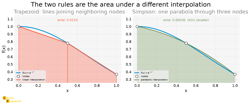
Note the detail that makes all the difference: the two rules use exactly the same three points. The cost is the same: three function evaluations. What changes is what is done with them. And the gain is forty-three-fold.
It might seem that fitting a parabola would be more expensive than joining two points with a line. It is not. Simpson’s rule, once the algebra is done, is a weighted average of the values at the nodes:
$$\int_{x_0}^{x_2} f(x) dx \approx \frac{h}{3}\left[f(x_0) + 4f(x_1) + f(x_2)\right]$$The coefficients \(1, 4, 1\) are already the result of integrating the parabola. Nobody needs to solve a system to find it at run time: the closed formula was derived once (Kepler already used it in 1615, and Simpson popularized it in the eighteenth century) and holds forever. It is the same economy as the trapezoid rule, whose weights are \(1, 1\).
The Difference Between \(O(h^2)\) and \(O(h^4)\) #
The exponents in the table above are not decoration. They say exactly how much you gain by spending more points, and the difference between \(2\) and \(4\) is large:
import numpy as np
from scipy import integrate


def test_func(t):
    return np.exp(-(t**2))


EXACT_AREA = 0.746824132812427

print(f"{'n':>6} {'h':>10} {'trapezoid err':>15} {'Simpson err':>14}")
for n in (4, 8, 16, 32, 64, 128, 256):
    xs = np.linspace(0, 1, n + 1)
    ys = test_func(xs)
    trap_err = abs(integrate.trapezoid(ys, xs) - EXACT_AREA)
    simp_err = abs(integrate.simpson(ys, x=xs) - EXACT_AREA)
    print(f"{n:>6} {xs[1] - xs[0]:>10.5f} {trap_err:>15.2e} {simp_err:>14.2e}")
n h trapezoid err Simpson err
4 0.25000 3.84e-03 3.12e-05
8 0.12500 9.59e-04 1.99e-06
16 0.06250 2.40e-04 1.25e-07
32 0.03125 5.99e-05 7.79e-09
64 0.01562 1.50e-05 4.87e-10
128 0.00781 3.74e-06 3.05e-11
256 0.00391 9.36e-07 1.90e-12Look at the ratios between consecutive rows. Each time \(n\) doubles (and so \(h\) is halved), the trapezoid error drops by 4 (\(=2^2\)) and the Simpson error by 16 (\(=2^4\)):
import numpy as np
from scipy import integrate


def test_func(t):
    return np.exp(-(t**2))


EXACT_AREA = 0.746824132812427

trap_errors, simp_errors = [], []
for n in (4, 8, 16, 32, 64, 128, 256):
    xs = np.linspace(0, 1, n + 1)
    ys = test_func(xs)
    trap_errors.append(abs(integrate.trapezoid(ys, xs) - EXACT_AREA))
    simp_errors.append(abs(integrate.simpson(ys, x=xs) - EXACT_AREA))
trap_errors, simp_errors = np.array(trap_errors), np.array(simp_errors)

print("ratio between consecutive errors:")
print("  trapezoid (expected 4  = 2²):", np.round(trap_errors[:-1] / trap_errors[1:], 2))
print("  Simpson   (expected 16 = 2⁴):", np.round(simp_errors[:-1] / simp_errors[1:], 2))
ratio between consecutive errors:
trapezoid (expected 4 = 2²): [4.01 4. 4. 4. 4. 4. ]
Simpson (expected 16 = 2⁴): [15.72 15.95 15.99 16. 16. 16. ]This is the same reading of the order of error that the article on numerical derivatives made for finite differences, and it is worth checking the pattern on a log-log plot, where a power law becomes a straight line:
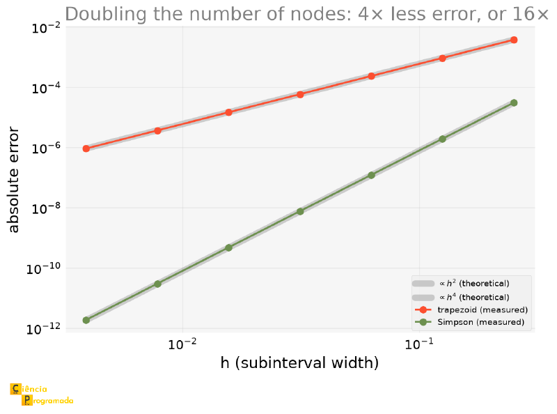
The table above is clean because the function is smooth and the interval is well chosen. With few nodes, and on an interval that contains an inflection point, Simpson can come out worse than the trapezoid.
In the case of \(e^{-x^2}\), the inflection is at \(x = 1/\sqrt{2} \approx 0.707\). Integrating over \([0, 2]\) with only two subintervals, the parabola tries to follow a curvature that changes sign midway, and Simpson’s error ends up ten times larger than the trapezoid’s: \(0.052\) against \(0.005\).
The \(O(h^4)\) order is an asymptotic result: it describes what
happens when \(h\) gets small enough, not a guarantee for any \(h\).
That is why adaptive quad is the default choice: it subdivides until the
asymptotic behavior actually holds, instead of trusting a fixed mesh
chosen at random.
Infinities and Peaks: Where quad Shines and Where It Fails
#
Infinite Limits #
np.inf is accepted as an integration limit, and quad internally makes a
change of variable that brings the infinity into a finite interval:
import numpy as np
from scipy import integrate

v_inf, e_inf = integrate.quad(lambda t: np.exp(-(t**2)), -np.inf, np.inf)
print(f"∫ e^(-x²) dx over the whole line = {v_inf:.12f}")
print(f"                    √π           = {np.sqrt(np.pi):.12f}")
∫ e^(-x²) dx over the whole line = 1.772453850906
√π = 1.772453850906Twelve correct digits on an integral over the entire line. It is worth noting what this means in practice: don’t truncate the tail by hand. The temptation to integrate from \(-10\) to \(10\) “because the rest is negligible” trades an exact result for an error you did not control. The figure below quantifies that error for the decaying exponential:
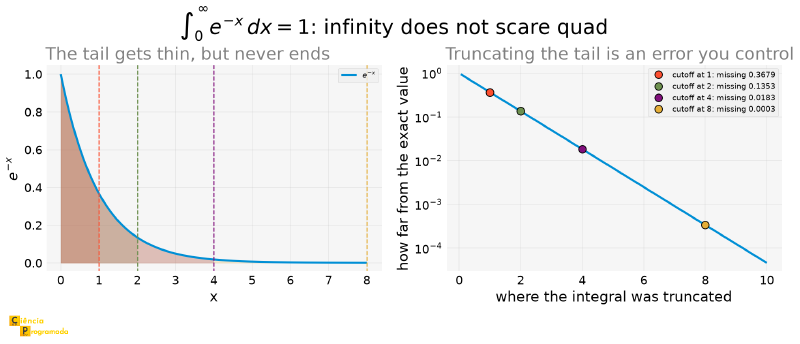
Truncating at \(x = 1\) loses \(37\%\) of the integral; at \(x = 2\), still \(13.5\%\); only at \(x = 8\) does the error drop to \(0.03\%\). These are numbers far too large for a “negligible” estimated by eye.
The Peak That quad Can’t See
#
All this competence has a limit, and it is important enough to deserve a scare:
quad can return zero with an estimated error of zero
Adaptive quadrature decides where to subdivide based on what it has already seen. If the first sampling of the interval does not touch the region where the function is nonzero, there is no large error to detect, and the algorithm concludes, with full confidence, that the integral is zero.
import numpy as np
from scipy import integrate

WIDTH = 1e-4
peak_func = lambda t: np.exp(-((t - 0.7) / WIDTH) ** 2)  # extremely narrow peak at 0.7
exact_area = WIDTH * np.sqrt(np.pi)

for kwargs, label in (
    ({}, "plain quad"),
    ({"points": [0.7]}, "points=[0.7]"),
    ({"points": [0.7 - 10 * WIDTH, 0.7 + 10 * WIDTH]}, "points around the peak"),
):
    v, e = integrate.quad(peak_func, 0, 1, **kwargs)
    actual_error = abs(v - exact_area) / exact_area * 100
    print(f"{label:>24}: {v:.6e}  est. error {e:.1e}  ACTUAL error {actual_error:7.3f}%")
print(f"{'exact':>24}: {exact_area:.6e}")
plain quad: 0.000000e+00 est. error 0.0e+00 ACTUAL error 100.000%
points=[0.7]: 6.524753e-22 est. error 1.3e-21 ACTUAL error 100.000%
points around the peak: 1.772454e-04 est. error 1.8e-10 ACTUAL error 0.000%
exact: 1.772454e-04The first line is the nightmare: result \(0\), estimated error \(0\). Total confidence in an answer that is one hundred percent wrong.
The second line shows that the obvious fix is not enough. The points
parameter tells quad where to break the interval, but breaking exactly at
\(0.7\) puts the peak on the edge of the two subintervals, and the
Gauss-Kronrod nodes are interior points of each panel: none falls exactly
on the edge, and the one closest to it is still too far away to see so
narrow a peak. The peak remains invisible.
The third line is the correct use: points surrounding the region of
interest, not pointing at it. Then the peak falls in the middle of a
subinterval and the error goes to zero.
The practical moral: know your function before integrating it. A quick plot of the integrand costs seconds and reveals any fine structure that the quadrature might skip. No adaptive algorithm can find what it never sampled.
A Family of Integrals at Once #
When the integrand returns a vector instead of a scalar, quad_vec solves
all the components at once, sharing the evaluations:
import numpy as np
from scipy import integrate

alphas = np.array([0.5, 1.0, 2.0, 4.0])
res, err = integrate.quad_vec(lambda t: np.exp(-alphas * t**2), 0, np.inf)

for a, v in zip(alphas, res):
    print(f"a={a:4.1f}: {v:.10f}   √(π/a)/2 = {np.sqrt(np.pi / a) / 2:.10f}")
a= 0.5: 1.2533141373 √(π/a)/2 = 1.2533141373
a= 1.0: 0.8862269255 √(π/a)/2 = 0.8862269255
a= 2.0: 0.6266570687 √(π/a)/2 = 0.6266570687
a= 4.0: 0.4431134627 √(π/a)/2 = 0.4431134627Integrating a Table: There Is No Function to Integrate #
The previous cases had at least a function. Now the most common case in the lab: there are only numbers. A chromatograph recorded signal against time; a datalogger recorded power against time; a stopwatch recorded position against time. There is no expression to differentiate or integrate: there is a table.
Here trapezoid and simpson stop being a didactic curiosity and become
the only option, because they work directly on arrays:
| Function | What it does |
|---|---|
integrate.trapezoid(y, x) |
Trapezoid rule over the given points |
integrate.simpson(y, x=x) |
Simpson’s rule over the given points |
integrate.cumulative_trapezoid(y, x, initial=0) |
The cumulative integral, returns an array, not a number |
None of them treats arbitrary spacing as a problem: the x vector can be
irregular, which is normal in real data.
Closing the Circle: Usain Bolt’s Race #
The article on numerical derivatives took Usain Bolt’s passing times in the Berlin final (2009), the position at every \(10\) m, and differentiated them to estimate the instantaneous velocity. Now we go the other way: integrating that velocity should reconstruct the position, and the integral over the whole race must give \(100\) m.
Let’s see if it does:
import numpy as np
from scipy import integrate

bolt_distance = np.arange(0, 101, 10)  # m, splits every 10 m
bolt_time = np.array([0, 1.89, 2.88, 3.78, 4.64, 5.47,
                      6.29, 7.10, 7.92, 8.75, 9.58])  # s

bolt_velocity = np.gradient(bolt_distance, bolt_time)   # from the previous article

trap_dist = integrate.trapezoid(bolt_velocity, bolt_time)
simp_dist = integrate.simpson(bolt_velocity, x=bolt_time)
print(f"actual distance: 100 m")
print(f"  integrating the velocity (trapezoid): {trap_dist:.3f} m")
print(f"  integrating the velocity (Simpson):   {simp_dist:.3f} m")
actual distance: 100 m
integrating the velocity (trapezoid): 102.230 m
integrating the velocity (Simpson): 102.055 mIt doesn’t: \(2.23\) m too many, more than two percent, over a course whose two endpoints are known exactly.
This is the kind of result worth more than a perfect closure, because it has
a locatable cause. Using cumulative_trapezoid to see where the error is
born:
import numpy as np
from scipy import integrate

bolt_distance = np.arange(0, 101, 10)  # m, splits every 10 m
bolt_time = np.array([0, 1.89, 2.88, 3.78, 4.64, 5.47,
                      6.29, 7.10, 7.92, 8.75, 9.58])  # s

bolt_velocity = np.gradient(bolt_distance, bolt_time)   # from the previous article

cum_dist = integrate.cumulative_trapezoid(bolt_velocity, bolt_time, initial=0)
for t, measured, integrated in zip(bolt_time, bolt_distance, cum_dist):
    print(f"t={t:5.2f}s  measured={measured:5.1f} m  integrated={integrated:7.3f} m"
          f"  difference={integrated - measured:+6.3f} m")
t= 0.00s measured= 0.0 m integrated= 0.000 m difference=+0.000 m
t= 1.89s measured= 10.0 m integrated= 12.983 m difference=+2.983 m
t= 2.88s measured= 20.0 m integrated= 22.426 m difference=+2.426 m
t= 3.78s measured= 30.0 m integrated= 32.329 m difference=+2.329 m
t= 4.64s measured= 40.0 m integrated= 42.312 m difference=+2.312 m
t= 5.47s measured= 50.0 m integrated= 52.257 m difference=+2.257 m
t= 6.29s measured= 60.0 m integrated= 62.258 m difference=+2.258 m
t= 7.10s measured= 70.0 m integrated= 72.198 m difference=+2.198 m
t= 7.92s measured= 80.0 m integrated= 82.199 m difference=+2.199 m
t= 8.75s measured= 90.0 m integrated= 92.230 m difference=+2.230 m
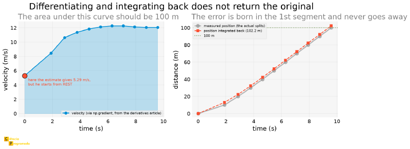
t= 9.58s measured=100.0 m integrated=102.230 m difference=+2.230 mThe right-hand column gives away the culprit. The entire error, almost three meters, shows up already in the first segment, between the starting gun and the \(10\) m mark. After that it hardly changes: the difference oscillates between \(2.20\) and \(2.43\) m until the end of the race.
And the reason lies in the velocity estimated at time zero:
import numpy as np

bolt_distance = np.arange(0, 101, 10)  # m, splits every 10 m
bolt_time = np.array([0, 1.89, 2.88, 3.78, 4.64, 5.47,
                      6.29, 7.10, 7.92, 8.75, 9.58])  # s

bolt_velocity = np.gradient(bolt_distance, bolt_time)   # from the previous article

print("estimated velocity at each mark (m/s):", np.round(bolt_velocity, 2))
estimated velocity at each mark (m/s): [ 5.29 8.45 10.63 11.38 11.84 12.12 12.27 12.27 12.12 12.05 12.05]\(5.29\) m/s at the start of the race. But Bolt starts from rest: the
actual velocity at \(t = 0\) is exactly zero. At the edge of the array,
np.gradient has no point on the left to make a central difference, and
falls back on a one-sided, first-order difference over an interval of
\(1.89\) s. Precisely the stretch in which the athlete accelerates the
hardest in the entire race. The estimate returns something close to the
average velocity of the stretch, not the initial one, and integrating that
average from \(t = 0\) inflates the area.
The figure shows both sides of the problem:
What just happened holds as a general rule, because it is a common trap in data processing.
In calculus, the fundamental theorem guarantees that differentiating and integrating are inverse operations. Numerically, they are not. Each one introduces its own error, and the errors do not cancel: they add up.
Worse: integration is a cumulative operation. An error made at the first point does not stay at the first point: it is carried, unchanged, through all the rest of the computation. That is exactly what the table showed: the deviation of \(+2.98\) m was born in the first segment and never left.
When you need both, prefer measuring the quantity you care about to differentiating or integrating it from another. And if there is no choice, use the boundary conditions you know (here, \(v(0) = 0\)) as a check, not as a fix: forcing \(v(0) = 0\) in this case takes the result to \(97.23\) m, missing in the other direction. The data are too coarse at the start for any pointwise adjustment to solve it.
Chemistry: Two Everyday Integrals #
In the two examples below, the integral is the definition of the quantity we want, not an exercise.
Enthalpy Change: \(\int C_p dT\) #
The heat capacity of a gas is not constant: it grows with temperature, and reference tables give \(C_p\) as a polynomial in \(T\). The heat needed to warm one mole from \(T_1\) to \(T_2\) at constant pressure is
$$ \Delta H = \int_{T_1}^{T_2} C_p(T) dT $$
Example 1: Heating CO₂ from 25 °C to 727 °C
Statement: For gaseous \(CO_2\), \(C_p(T) = 22.243 + 5.977\times10^{-2}\ T - 3.499\times10^{-5}\ T^2\) in J/(mol·K), with \(T\) in kelvin. Compute \(\Delta H\) when heating from \(298.15\) K to \(1000\) K.
Solution:
from scipy import integrate


def cp_co2(T):
    return 22.243 + 5.977e-2 * T - 3.499e-5 * T**2


delta_H, err = integrate.quad(cp_co2, 298.15, 1000.0)
print(f"ΔH = {delta_H:.1f} J/mol = {delta_H / 1000:.2f} kJ/mol")
print(f"estimated error: {err:.1e} J/mol")
ΔH = 31485.5 J/mol = 31.49 kJ/mol
estimated error: 3.5e-10 J/molThis is a case where the antiderivative exists and is trivial: it is a degree-3 polynomial. It is worth checking against SymPy:
import sympy as sp

T = sp.symbols("T")
cp_sym = 22.243 + 5.977e-2 * T - 3.499e-5 * T**2
print("SymPy:", float(sp.integrate(cp_sym, (T, 298.15, 1000.0))))
SymPy: 31485.45630238881Agreement down to the last digit. When both routes are available, using both is the cheapest form of validation there is.
What interests us here is the comparison with the shortcut that every undergraduate course teaches first, which is to assume constant \(C_p\), evaluated at the initial temperature:
from scipy import integrate


def cp_co2(T):
    return 22.243 + 5.977e-2 * T - 3.499e-5 * T**2


delta_H, _ = integrate.quad(cp_co2, 298.15, 1000.0)

delta_H_constant = cp_co2(298.15) * (1000.0 - 298.15)
print(f"assuming constant Cp at {cp_co2(298.15):.2f} J/(mol·K): "
      f"{delta_H_constant / 1000:.2f} kJ/mol")
print(f"error of the approximation: {(delta_H_constant - delta_H) / delta_H * 100:+.1f}%")
assuming constant Cp at 36.95 J/(mol·K): 25.94 kJ/mol
error of the approximation: -17.6%Almost eighteen percent too low. Over a \(700\) K range, the \(C_p\) of \(CO_2\) grows enough that freezing it at the initial value stops being an approximation and becomes a gross error. The integral costs one line; the approximation costs eighteen percent.
Expansion Work: \(\int P dV\) #
The work done by a gas expanding reversibly is the area under the \(P(V)\) curve:
$$ W = \int_{V_1}^{V_2} P(V) dV $$For an ideal gas, \(P = RT/V\), the antiderivative is the logarithm and the result is the classic formula \(W = RT\ln(V_2/V_1)\). But the article on chemistry and engineering equations showed that real gases at high pressures do not follow the ideal law; they follow, much more faithfully, the van der Waals equation:
$$ P(V) = \frac{RT}{V - b} - \frac{a}{V^2} $$And this one, integrated, also has an elementary antiderivative, but nobody needs to find it to get the number:
Example 2: Isothermal expansion of CO₂, ideal versus real
Statement: One mole of \(CO_2\) expands isothermally at \(300\) K from \(0.1\) to \(2.0\) L/mol. Compare the work predicted by the ideal model with that predicted by van der Waals (\(a = 3.640\) L²·atm/mol², \(b = 0.04267\) L/mol).
Solution:
import numpy as np
from scipy import integrate

R_GAS = 0.082057   # L·atm/(mol·K)
A_VDW, B_VDW = 3.640, 0.04267
T_EXP = 300.0
V1, V2 = 0.1, 2.0


def p_ideal(V):
    return R_GAS * T_EXP / V


def p_vdw(V):
    return R_GAS * T_EXP / (V - B_VDW) - A_VDW / V**2


w_ideal, _ = integrate.quad(p_ideal, V1, V2)
w_vdw, err = integrate.quad(p_vdw, V1, V2)

print(f"ideal gas:     {w_ideal:8.4f} L·atm/mol")
print(f"  (analytic:   {R_GAS * T_EXP * np.log(V2 / V1):8.4f}  = RT ln(V2/V1))")
print(f"van der Waals: {w_vdw:8.4f} L·atm/mol   (estimated error {err:.1e})")
print(f"difference: {(w_vdw - w_ideal) / w_ideal * 100:+.1f}%")
ideal gas: 73.7462 L·atm/mol
(analytic: 73.7462 = RT ln(V2/V1))
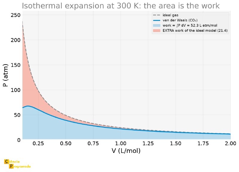
van der Waals: 52.3310 L·atm/mol (estimated error 5.2e-07)
difference: -29.0%Twenty-nine percent difference. And it is no mere model detail: at \(0.1\) L/mol the \(CO_2\) is compressed to the point where the attractive forces between molecules (the \(-a/V^2\) term) push the pressure well below what the ideal law predicts. Less pressure, less area, less work.
The plot makes the difference literally visible as an area:
Points of Attention #
The three cheapest checks, in order of cost:
- Look at the error estimate.
quadreturns it for free. An estimated error of the order of the result itself is a red flag. - Plot the integrand. Seconds of work, and it reveals narrow peaks, singularities and oscillations that any adaptive method may skip.
- Check against an independent route. If SymPy closes it, compare. If there is a known limiting case (the ideal gas, here), compare with it.
Simpson’s rule consumes the nodes three at a time, with overlap, which
requires an even number of subintervals (that is, an odd number of
points). With an odd number of subintervals, scipy.integrate.simpson
does not raise an error: it applies a correction on the last interval,
which has a lower order of error than the rest. The result remains usable,
but the \(O(h^4)\) convergence no longer holds. When the order matters,
make sure len(x) is odd.
trapezoid and simpson don’t estimate error
Unlike quad, the rules over tabulated data return only the value. There
is no way to ask them for an error estimate, because there is no way to
refine the mesh: the data are what they are. The practical way to estimate
the error in this case is to compare trapezoid with simpson: if the two
agree to many digits, the mesh is fine enough for the curvature of the
function. That is what happened with Bolt (\(102.230\) against
\(102.055\)): the two agree, and yet both are \(2\%\) away from the
right value. Agreement between methods attests that the mesh is
sufficient, not that the input data are correct.
Summary Table #
| Tool | Use | Remark |
|---|---|---|
sympy.integrate |
First attempt, always | When it closes, the exact answer is better than any approximation |
scipy.integrate.quad |
Integral of a function of one variable | Returns (value, error_estimate); the estimate is conservative |
quad(..., a, np.inf) |
Improper integrals | Better than truncating the tail by hand: the truncation error is large and avoidable |
quad(..., points=[...]) |
Fine structure in the integrand | Surround the critical region, don’t point at it |
scipy.integrate.quad_vec |
A family of integrals at once | Integrand returns a vector; shares evaluations |
integrate.trapezoid(y, x) |
Tabulated data | Error \(O(h^2)\); accepts irregular spacing |
integrate.simpson(y, x=x) |
Tabulated data | Error \(O(h^4)\); requires an even number of subintervals |
integrate.cumulative_trapezoid |
Cumulative integral | Returns an array; essential to locate where an error is born |
| Concept | Remark |
|---|---|
| Liouville’s theorem | \(\int e^{-x^2}dx\) has no elementary antiderivative: it is a theorem, not a software limitation |
| Special functions | erf, Si, Ei are names for integrals that don’t close; they live in scipy.special |
| Order of error | Doubling the nodes: trapezoid improves \(4\times\), Simpson \(16\times\), but only in the asymptotic regime |
| Adaptive quadrature | Subdivides where the error is large; does not find what it never sampled |
| Cumulative error | Integration carries forward the error made at the start, without damping it |
| Differentiating × integrating | Numerically they are not inverses: the errors add up, they don’t cancel |
Next Steps #
The integrals in this article all have the same structure: the integrand is known beforehand. A function that can be evaluated at any point, or a table already measured. Given that, computing the area is a solved problem.
But the most interesting case in applied science is not that one. When the rate of change of a quantity depends on the current value of that same quantity (the speed of a reaction depends on how much reactant is still left, the current depends on the charge already accumulated in the capacitor), there is no integrand to tabulate before starting. Each step depends on the previous one.
This stops being an integral and becomes a differential equation, the
subject of the
next article in the series.
And the instrument there, solve_ivp, with its adaptive step, is a close
relative of the adaptive quad seen here: the same idea of spending effort
where the problem is hard, applied to a problem in which the answer is built
as you go along.


