

A lab technician watches the temperature of a reactor on a datalogger (a device that automatically records measurements over time): a sequence of numbers read every few seconds, with no formula attached. At some point they need to answer a very concrete question: “is the temperature rising too fast right now?”. Mathematically, that question is a derivative. But there is no \(f(x)\) to differentiate. There are only numbers in a table.
SymPy computes derivatives of any closed-form expression with a single function call, but it has no answer for this problem: there is no “symbolic derivative of a table”. This is exactly where numerical derivatives come in: techniques that estimate the rate of change of a function from sampled values alone, with or without a formula behind them.
Why Do Numerical Derivatives Matter? #
- Physics and sensor engineering: accelerometers, position sensors and oscilloscopes deliver sequences of readings over time, and instantaneous velocity and acceleration exist only as numerical derivatives of that data.
- Chemistry and reaction kinetics: the rate of a reaction at a given instant is the derivative of the concentration with respect to time, estimated from bench measurements, not from a formula known a priori.
- Control and signal processing: a PID controller (proportional-integral-derivative, a classic automatic control architecture) uses the derivative of the system error in real time, computed on sampled and often noisy data.
- Numerical optimization: when the objective function has no analytic gradient available (or is too expensive to differentiate symbolically), optimizers fall back on numerical approximations of the derivative, a topic that will return in the optimization article of this series.
From Symbolic diff to the Numerical Difference
#
The SymPy derivatives article
used the function \(f(x) = x^3\) to introduce diff: the exact derivative,
\(f^{\prime}(x) = 3x^2\), evaluated at \(x_0 = 2\), is \(12\). The idea
behind any numerical derivative is to directly approximate the definition of
the derivative, the limit of a difference quotient, without actually taking
the limit, using a small \(h\) instead of \(h \to 0\):
This is the central difference. Applying it with a few decreasing values of \(h\) and comparing with the exact value:
import sympy as sp

x = sp.symbols("x")
f_sym = x**3
f_num = sp.lambdify(x, f_sym)
df_exact = sp.lambdify(x, sp.diff(f_sym, x))

x0 = 2.0
exact_value = df_exact(x0)


def central_difference(f, x0, h):
    return (f(x0 + h) - f(x0 - h)) / (2 * h)


for h in [1e-1, 1e-2, 1e-3, 1e-4]:
    approx = central_difference(f_num, x0, h)
    error = abs(approx - exact_value)
    print(f"h={h:.0e}  approximation={approx:.10f}  error={error:.2e}")
h=1e-01 approximation=12.0100000000 error=1.00e-02
h=1e-02 approximation=12.0001000000 error=1.00e-04
h=1e-03 approximation=12.0000010000 error=1.00e-06
h=1e-04 approximation=12.0000000100 error=1.00e-08Each time \(h\) shrinks by a factor of 10, the error drops by a factor of about 100. That is the signature of a second-order method, \(O(h^2)\), which the next section explains.
The same idea rebuilds the tangent line from that article,
\(f(x) = \frac12 x^2\) at \(x_0 = 1\), without using diff even once:
import numpy as np


def central_difference(f, x0, h):
    return (f(x0 + h) - f(x0 - h)) / (2 * h)


def f_tangent(x):
    return 0.5 * x**2


x0_tangent = 1.0
fp_tangent = central_difference(f_tangent, x0_tangent, h=1e-5)


def tangent_line(x):
    return f_tangent(x0_tangent) + fp_tangent * (x - x0_tangent)


print("numerical f'(1):", fp_tangent)
numerical f'(1): 1.000000000001Practically \(1.0\), the exact value. The following figure shows the parabola and the tangent line built entirely from this numerical derivative:
import matplotlib.pyplot as plt
import numpy as np


def central_difference(f, x0, h):
    return (f(x0 + h) - f(x0 - h)) / (2 * h)


def f_tangent(x):
    return 0.5 * x**2


x0_tangent = 1.0
fp_tangent = central_difference(f_tangent, x0_tangent, h=1e-5)


def tangent_line(x):
    return f_tangent(x0_tangent) + fp_tangent * (x - x0_tangent)


xs = np.linspace(-1, 3, 200)

fig, ax = plt.subplots()
ax.plot(xs, f_tangent(xs), label=r"$f(x) = \frac{1}{2}x^2$")
ax.plot(xs, tangent_line(xs), "--", label="tangent line (numerical derivative)")
ax.plot(x0_tangent, f_tangent(x0_tangent), "o", color="black")
ax.set_xlabel("x")
ax.set_ylabel("y")
ax.legend()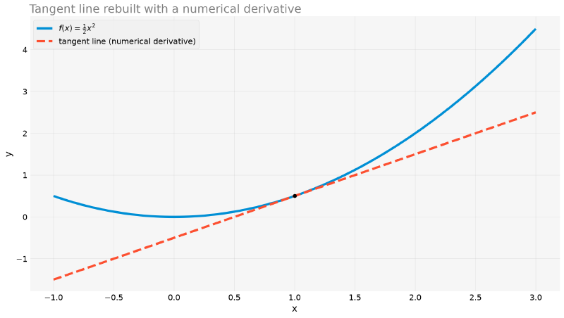
The Finite Difference Formulas #
The central difference is not the only option, and it is worth knowing the other two to understand why it is usually the default choice.
- Forward: \(\displaystyle f^{\prime}(x_0) \approx \frac{f(x_0+h) - f(x_0)}{h}\), error \(O(h)\)
- Backward: \(\displaystyle f^{\prime}(x_0) \approx \frac{f(x_0) - f(x_0-h)}{h}\), error \(O(h)\)
- Central: \(\displaystyle f^{\prime}(x_0) \approx \frac{f(x_0+h) - f(x_0-h)}{2h}\), error \(O(h^2)\)
Forward and backward use only one “side” of \(x_0\); the central uses both, and this symmetry cancels the first-order error term of the Taylor expansion, which is why it converges much faster.
That last sentence deserves the five lines of algebra that justify it, because without them “\(O(h^2)\)” is a memorized label. Everything comes from expanding \(f\) in a Taylor series on both sides of \(x_0\):
$$ f(x_0+h) = f + hf' + \frac{h^2}{2}f'' + \frac{h^3}{6}f''' + \cdots $$$$ f(x_0-h) = f - hf' + \frac{h^2}{2}f'' - \frac{h^3}{6}f''' + \cdots $$Forward. Solving the first one for \(f^{\prime}\):
$$ \frac{f(x_0+h) - f(x_0)}{h} = f' + \frac{h}{2}f'' + O(h^2) $$A term proportional to \(h\) is left over, hence the \(O(h)\).
Central. Subtracting the second from the first, all the even-power terms cancel, including \(\frac{h^2}{2}f^{\prime\prime}\), which was the villain:
$$ f(x_0+h) - f(x_0-h) = 2hf' + \frac{h^3}{3}f''' + \cdots $$$$ \frac{f(x_0+h) - f(x_0-h)}{2h} = f' + \frac{h^2}{6}f''' + O(h^4) $$The first error term is now \(h^2\), and the next one is \(h^4\). The symmetry eliminates half of the Taylor series for free, and that is what makes the central difference look “smarter”.
It is worth seeing this with an \(h\) large enough for the lines to separate in the drawing. For \(f(x)=x^3\) at \(x_0=2\), with \(h = 0.9\):
def f(x):
    return x**3


x0, h = 2.0, 0.9
exact_derivative = 3 * x0**2

for name, approx in (
    ("forward", (f(x0 + h) - f(x0)) / h),
    ("backward", (f(x0) - f(x0 - h)) / h),
    ("central", (f(x0 + h) - f(x0 - h)) / (2 * h)),
):
    print(f"  {name:>11} = {approx:7.4f}   error = {abs(approx - exact_derivative):.4f}")
forward = 18.2100 error = 6.2100
backward = 7.4100 error = 4.5900
central = 12.8100 error = 0.8100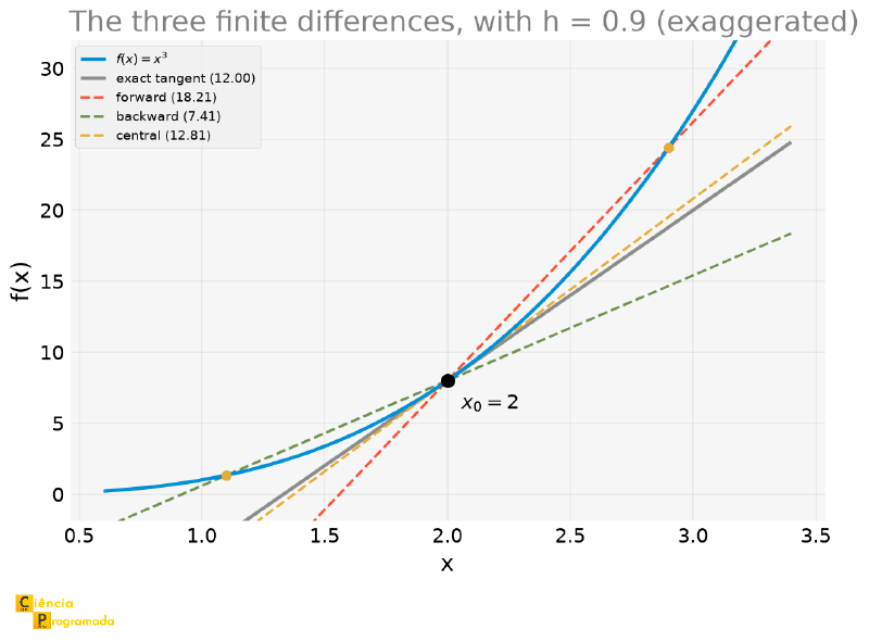
The figure shows the mechanism better than the algebra: the forward difference is off by \(+6.21\) and the backward by \(-4.59\), in opposite directions. The central is essentially the average of the two, and the two errors cancel almost entirely, leaving \(0.81\).
Repeating the same experiment for \(f(x) = x^3\) at \(x_0 = 2\) for the three formulas:
import sympy as sp

x = sp.symbols("x")
f_sym = x**3
f_num = sp.lambdify(x, f_sym)
df_exact = sp.lambdify(x, sp.diff(f_sym, x))

x0 = 2.0
exact_value = df_exact(x0)


def central_difference(f, x0, h):
    return (f(x0 + h) - f(x0 - h)) / (2 * h)


def forward_difference(f, x0, h):
    return (f(x0 + h) - f(x0)) / h


def backward_difference(f, x0, h):
    return (f(x0) - f(x0 - h)) / h


print(f"{'h':>10}  {'forward':>14}  {'backward':>14}  {'central':>14}")
for h in [1e-1, 1e-2, 1e-3, 1e-4]:
    ep = abs(forward_difference(f_num, x0, h) - exact_value)
    er = abs(backward_difference(f_num, x0, h) - exact_value)
    ec = abs(central_difference(f_num, x0, h) - exact_value)
    print(f"{h:>10.0e}  {ep:>14.2e}  {er:>14.2e}  {ec:>14.2e}")
h forward backward central
1e-01 6.10e-01 5.90e-01 1.00e-02
1e-02 6.01e-02 5.99e-02 1.00e-04
1e-03 6.00e-03 6.00e-03 1.00e-06
1e-04 6.00e-04 6.00e-04 1.00e-08| h | forward error | backward error | central error |
|---|---|---|---|
| \(10^{-1}\) | \(6.10 \times 10^{-1}\) | \(5.90 \times 10^{-1}\) | \(1.00 \times 10^{-2}\) |
| \(10^{-2}\) | \(6.01 \times 10^{-2}\) | \(5.99 \times 10^{-2}\) | \(1.00 \times 10^{-4}\) |
| \(10^{-3}\) | \(6.00 \times 10^{-3}\) | \(6.00 \times 10^{-3}\) | \(1.00 \times 10^{-6}\) |
| \(10^{-4}\) | \(6.00 \times 10^{-4}\) | \(6.00 \times 10^{-4}\) | \(1.00 \times 10^{-8}\) |
Forward and backward are off by a factor of \(\approx 10\) for each reduction of \(h\) by \(10\), the signature of \(O(h)\). The central is off by a factor of \(\approx 100\), \(O(h^2)\), confirming what the theory predicts.
Differentiating Tabulated Data: numpy.gradient
#
Formula in hand, the real problem (tabulated data, with no formula at all)
finally fits. numpy.gradient applies the central difference at the interior
points of an array (and the forward/backward difference at the edges, where
there is no neighbor on both sides) and accepts non-uniformly spaced
coordinates.
Example: Usain Bolt’s Velocity from the Splits
Statement: The article on Usain Bolt's record has Bolt’s cumulative times at each 10 m mark of the Berlin 2009 final: position every 10 m, non-uniformly spaced time. Estimate the instantaneous velocity at each mark.
Solution:
import numpy as np

bolt_distance = np.arange(0, 101, 10)  # m, splits every 10 m
bolt_time = np.array(
    [0, 1.89, 2.88, 3.78, 4.64, 5.47, 6.29, 7.10, 7.92, 8.75, 9.58]
)  # s

bolt_velocity = np.gradient(bolt_distance, bolt_time)
print("velocities (m/s):", np.round(bolt_velocity, 2))
print("maximum velocity:", np.round(bolt_velocity.max(), 2), "m/s")
velocities (m/s): [ 5.29 8.45 10.63 11.38 11.84 12.12 12.27 12.27 12.12 12.05 12.05]
maximum velocity: 12.27 m/sThe peak, \(12.27\) m/s, happens between 60 and 70 meters, consistent
with what is known about the race. In the original article, the velocity
came from fitting a cubic spline to the data and differentiating that
spline analytically (CubicSpline(...).derivative()), which gave a maximum
velocity of \(12.37\) m/s. Here, without fitting anything, applying a
finite difference directly to the raw points, the result is
\(0.10\) m/s away (\(< 1\%\)), good news: for a quick estimate,
numpy.gradient already delivers a result almost as good as a more
elaborate fit.
The following graph shows this evolution:
import matplotlib.pyplot as plt
import numpy as np

bolt_distance = np.arange(0, 101, 10)  # m, splits every 10 m
bolt_time = np.array(
    [0, 1.89, 2.88, 3.78, 4.64, 5.47, 6.29, 7.10, 7.92, 8.75, 9.58]
)  # s

bolt_velocity = np.gradient(bolt_distance, bolt_time)

fig, ax = plt.subplots()
ax.plot(bolt_time, bolt_velocity, "o-")
ax.set_xlabel("time (s)")
ax.set_ylabel("velocity (m/s)")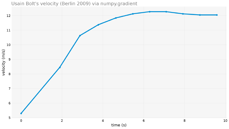
A Modern API: scipy.differentiate
#
For closed-form functions (not tabulated data), SciPy has an API dedicated to numerical derivatives, with automatic error estimation and stopping criterion, more robust than picking a single \(h\) by hand:
from scipy import differentiate

x0 = 2.0
res = differentiate.derivative(lambda x: x**3, x0)
print("f'(2):", res.df, " estimated error:", res.error, " evaluations:", res.nfev)
f'(2): 12.0 estimated error: 1.4210854715202004e-14 evaluations: 11scipy.misc.derivative was removed
Older versions of SciPy had scipy.misc.derivative, now completely
removed (not merely deprecated). Old code that still imports it breaks
with ImportError. The current alternative is
scipy.differentiate.derivative (seen above) or a manual central
difference like the ones in the previous sections.
The Step-Size Trade-off: Truncation × Rounding #
Back to the manual central difference: if the error falls with smaller \(h\), why not always choose a tiny \(h\)? Repeating the experiment with \(f(x)=x^3\) at \(x_0=2\), but sweeping \(h\) over a much wider range, from \(10^{-16}\) to \(10^{-1}\), reveals the answer:
import matplotlib.pyplot as plt
import numpy as np
import sympy as sp

x = sp.symbols("x")
f_sym = x**3
f_num = sp.lambdify(x, f_sym)
df_exact = sp.lambdify(x, sp.diff(f_sym, x))

x0 = 2.0
exact_value = df_exact(x0)


def central_difference(f, x0, h):
    return (f(x0 + h) - f(x0 - h)) / (2 * h)


hs = np.logspace(-16, -1, 200)
central_errors = np.array(
    [abs(central_difference(f_num, x0, h) - exact_value) for h in hs]
)

fig, ax = plt.subplots()
ax.loglog(hs, central_errors)
ax.set_xlabel("h")
ax.set_ylabel("absolute error")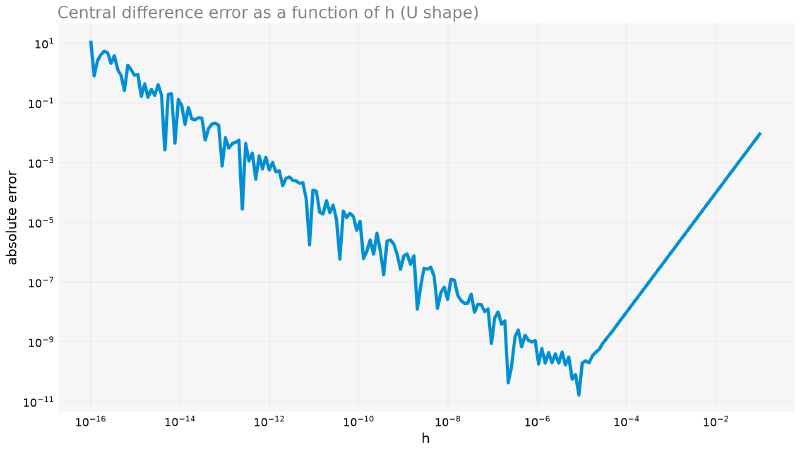
import numpy as np
import sympy as sp

x = sp.symbols("x")
f_sym = x**3
f_num = sp.lambdify(x, f_sym)
df_exact = sp.lambdify(x, sp.diff(f_sym, x))

x0 = 2.0
exact_value = df_exact(x0)


def central_difference(f, x0, h):
    return (f(x0 + h) - f(x0 - h)) / (2 * h)


hs = np.logspace(-16, -1, 200)
central_errors = np.array(
    [abs(central_difference(f_num, x0, h) - exact_value) for h in hs]
)

h_opt = hs[np.argmin(central_errors)]
print("approximately optimal h:", h_opt)
print("minimum error:", central_errors.min())
approximately optimal h: 8.50448934180267e-06
minimum error: 1.6351364706679306e-11For larger \(h\), the truncation error dominates: the very approximation of the derivative by a finite difference quotient, which the theory predicts as \(O(h^2)\). For \(h\) smaller than \(\approx 10^{-5}\) to \(10^{-6}\) (in this example, in double-precision floating point), the rounding error dominates: \(f(x_0+h)\) and \(f(x_0-h)\) become so close that the subtraction loses significant digits. The graph is not a curve decreasing to zero: it is a “U”, with an optimal \(h\) in the middle.
The “U” Is the Sum of Two Lines #
The shape is no mystery: it is two simple laws added together, each one dominating one side.
- Truncation. From the Taylor derivation, the error is \(\frac{h^2}{6}|f^{\prime\prime\prime}|\). For \(f = x^3\), \(f^{\prime\prime\prime} = 6\), so it is exactly \(h^2\).
- Rounding. Each evaluation of \(f\) carries a relative error \(\epsilon \approx 2.2\times10^{-16}\), hence an absolute error \(\epsilon|f|\). The subtraction in the numerator adds the two, and the division by \(2h\) amplifies: the error becomes \(\epsilon|f|/h\).
Differentiating and setting to zero, the minimum is at:
$$ h_{\text{opt}} = \sqrt[3]{\frac{\epsilon |f|}{2}} $$import numpy as np
import sympy as sp
x = sp.symbols("x")
f_sym = x**3
f_num = sp.lambdify(x, f_sym)
df_exact = sp.lambdify(x, sp.diff(f_sym, x))
x0 = 2.0
exact_value = df_exact(x0)
def central_difference(f, x0, h):
return (f(x0 + h) - f(x0 - h)) / (2 * h)
hs = np.logspace(-16, -1, 200)
central_errors = np.array(
[abs(central_difference(f_num, x0, h) - exact_value) for h in hs]
)
machine_eps = np.finfo(float).eps
h_theory = (machine_eps * abs(f_num(x0)) / 2) ** (1 / 3)
print(f"measured optimal h: {hs[np.argmin(central_errors)]:.3e}")
print(f"predicted optimal h: {h_theory:.3e}")measured optimal h: 8.504e-06
predicted optimal h: 9.612e-06Same order of magnitude, with a factor of 1.1 difference, which is good enough, because the rounding model is a rough estimate. And the exponent \(1/3\) stops being magical: it comes from balancing \(h^2\) against \(1/h\).
The following graph puts the three curves together, the measured error and the two theoretical terms:
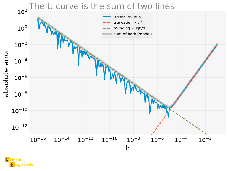
Two things to notice in the figure. First, the measured curve hugs each of the lines in its regime: the two-term model describes well what happens. Second, the left side is jagged and the right side is smooth: the truncation error is deterministic, but the rounding error depends on which bits are left over in each subtraction, and varies erratically. That is why the “optimal \(h\)” is, in practice, a region and not a point; it is not worth hunting for the exact value.
The Second Derivative Is Even More Fragile #
The same Taylor expansion gives the formula for the second derivative, this time adding the two expansions instead of subtracting:
Truncation error \(O(h^2)\), like the first derivative. This formula is used in the discretization of partial differential equations.
But the \(h^2\) in the denominator changes everything on the rounding side: instead of \(\epsilon|f|/h\), the error becomes \(\epsilon|f|/h^2\). The effect is visible in a clean case. For \(f = x^3\), the fourth derivative is zero, so the truncation vanishes and what remains is 100% rounding:
import sympy as sp

x = sp.symbols("x")
f_num = sp.lambdify(x, x**3)
x0 = 2.0

for h in (1e-1, 1e-2, 1e-3, 1e-4, 1e-5):
    d2 = (f_num(x0 + h) - 2 * f_num(x0) + f_num(x0 - h)) / h**2
    print(f"h={h:.0e}: f''={d2:.8f}   error={abs(d2 - 12):.2e}")
h=1e-01: f''=12.00000000 error=8.88e-15
h=1e-02: f''=12.00000000 error=2.80e-11
h=1e-03: f''=12.00000000 error=9.87e-10
h=1e-04: f''=12.00000028 error=2.82e-07
h=1e-05: f''=12.00000987 error=9.87e-06Each division of \(h\) by 10 multiplies the error by 100, the signature of \(1/h^2\). Notice that here the “best” \(h\) is the largest one tested, the opposite of intuition. For a function with a nonzero fourth derivative there would be a \(U\) again, but with the minimum at an \(h\) much larger than that of the first derivative.
When the Data Is Noisy #
The same U shape appears in another way when the data comes from a real measurement, with noise, and in that case the source of the problem stops being floating-point rounding and becomes the instrument.
import numpy as np

noise_sigma = 0.01


def noise_experiment(n_points, seed=7):
    rng = np.random.default_rng(seed + n_points)  # seed per call
    xs = np.linspace(0, 2 * np.pi, n_points)
    noise = rng.normal(0, noise_sigma, size=xs.shape)
    noisy_signal = np.sin(xs) + noise
    numerical_derivative = np.gradient(noisy_signal, xs)
    error = np.abs(numerical_derivative - np.cos(xs))
    return xs, noisy_signal, numerical_derivative, error


print(f"{'n points':>10}  {'h':>10}  {'mean error':>12}  {'max error':>12}")
for n in [20, 50, 200, 1000]:
    xs, _, _, error = noise_experiment(n)
    h = xs[1] - xs[0]
    print(f"{n:>10d}  {h:>10.4f}  {error.mean():>12.4f}  {error.max():>12.4f}")
n points h mean error max error
20 0.3307 0.0239 0.0618
50 0.1282 0.0412 0.1436
200 0.0316 0.1759 0.7145
1000 0.0063 0.8771 4.2044The signal is \(\sin(x)\) with a small Gaussian noise, \(\sigma = 0.01\), almost imperceptible to the naked eye. Even so, refining the grid makes the derivative worse: with \(1000\) points, the mean error (\(0.88\)) is already of the same order of magnitude as the amplitude of the cosine we want to recover, which is \(1\). In other words: the “signal” and the “error” end up with comparable sizes, and the derivative stops meaning much.
The reason is that the noise does not change in amplitude when \(h\) shrinks, but the real variation of the signal between two neighboring points does; so, as the points get closer, the noise comes to dominate. And this can be predicted before running. In the central difference, the noise of the two samples enters divided by \(2h\):
$$ \sigma_{\text{derivative}} \approx \frac{\sqrt{2}\sigma}{2h} = \frac{\sigma}{\sqrt{2} h} $$With \(1000\) points in \([0, 2\pi]\), we have \(h \approx 0.0063\) and \(\sigma = 0.01\), which gives \(\sigma_{\text{derivative}} \approx 1.12\). The mean absolute error of a Gaussian is \(\sqrt{2/\pi} \approx 0.80\) times its standard deviation, that is, \(\approx 0.90\), matching the \(0.88\) measured. Notice the \(h\) in the denominator: the derivative error grows when the grid is refined, exactly the opposite of what happens with the truncation error.
import matplotlib.pyplot as plt
import numpy as np

noise_sigma = 0.01


def noise_experiment(n_points, seed=7):
    rng = np.random.default_rng(seed + n_points)  # seed per call
    xs = np.linspace(0, 2 * np.pi, n_points)
    noise = rng.normal(0, noise_sigma, size=xs.shape)
    noisy_signal = np.sin(xs) + noise
    numerical_derivative = np.gradient(noisy_signal, xs)
    error = np.abs(numerical_derivative - np.cos(xs))
    return xs, noisy_signal, numerical_derivative, error


xs_fine, signal_fine, deriv_fine, _ = noise_experiment(200)

fig, (ax1, ax2) = plt.subplots(2, 1, sharex=True, figsize=(8, 6))
ax1.plot(xs_fine, signal_fine, "o", color="C0", markersize=3, alpha=0.6,
         label="measured signal (noisy)", zorder=1)
ax1.plot(xs_fine, np.sin(xs_fine), color="C1", linewidth=2, label=r"true $\sin(x)$", zorder=2)
ax1.legend()

ax2.plot(xs_fine, deriv_fine, color="C0", label="numerical derivative")
ax2.plot(xs_fine, np.cos(xs_fine), color="C1", linewidth=2, label=r"true $\cos(x)$")
ax2.set_xlabel("x")
ax2.legend()
The following figure compares the measured signal with the real one (top) and the numerical derivative with the real derivative (bottom):
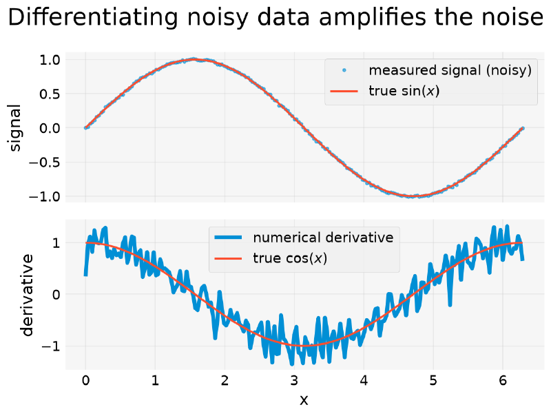
In the previous section, the “U” came from floating-point rounding, a problem that goes away if \(h\) is larger. Here, it comes from measurement noise, which no \(h\) eliminates by itself: refining the grid only concentrates more noise per unit of \(h\). In practice, noisy data sometimes calls for smoothing before differentiating, or a deliberately larger \(h\), the opposite of the “more points is always better” instinct.
Application: Reaction Rate from Concentration Data #
One last application, leaning toward chemistry: a kinetics experiment measures the concentration of a reactant at times chosen by the experimenter (non-uniformly spaced), without assuming beforehand what the rate law of the reaction is.
Example: Instantaneous Reaction Rate Without Knowing the Kinetics
Statement: A reaction is followed through 11 concentration measurements between \(t=0\) and \(t=30\) min. Estimate the instantaneous reaction rate, \(-dC/dt\), at each measured time, without assuming the order of the reaction.
Solution:
import numpy as np

kinetics_time = np.array([0, 2, 4, 6, 8, 10, 12, 15, 20, 25, 30])  # min
measured_concentration = np.array(
    [2.02, 1.456, 1.102, 0.807, 0.598, 0.444, 0.31, 0.208, 0.091, 0.08, 0.024]
)  # mol/L

instantaneous_rate = -np.gradient(measured_concentration, kinetics_time)
print("rate (mol/L/min):", np.round(instantaneous_rate, 4))
rate (mol/L/min): [0.282 0.2295 0.1622 0.126 0.0908 0.072 0.0538 0.03 0.0128 0.0067
0.0112]With only the measured data and numpy.gradient, without fitting any
kinetic model, we already get the rate at each point, a first step of
chemical kinetics analysis. Only after having this curve does it make
sense to ask whether it is compatible with a 1st-order law, a 2nd-order
one, or something else.
To check, I need to “cheat”. Since the concentration data above was simulated, I know the real relationship behind it: \(C(t) = C_0 e^{-kt}\), with \(k=0.15\) min\(^{-1}\) and \(C_0=2\) mol/L, something that, with real bench data, I could never know beforehand. I use this real relationship only to generate a continuous reference curve, evaluated on a fine time grid (not only at the 11 measured instants, otherwise I fall into the same problem of connecting a few points with straight lines from the previous section), and compare it with the estimated rate:
import matplotlib.pyplot as plt
import numpy as np

kinetics_time = np.array([0, 2, 4, 6, 8, 10, 12, 15, 20, 25, 30])  # min
measured_concentration = np.array(
    [2.02, 1.456, 1.102, 0.807, 0.598, 0.444, 0.31, 0.208, 0.091, 0.08, 0.024]
)  # mol/L

instantaneous_rate = -np.gradient(measured_concentration, kinetics_time)

time_fine = np.linspace(0, 30, 200)
k_true, C0_true = 0.15, 2.0  # known only because the data is synthetic
true_rate_continuous = k_true * C0_true * np.exp(-k_true * time_fine)

fig, ax = plt.subplots()
ax.plot(kinetics_time, instantaneous_rate, "o", label="estimated rate (numpy.gradient)")
ax.plot(time_fine, true_rate_continuous, "--", label=r"$k \cdot C_0 e^{-kt}$ (check)")
ax.set_xlabel("t (min)")
ax.set_ylabel("reaction rate (mol/L/min)")
ax.legend()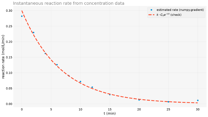
The rate estimated by finite differences, computed without knowing \(k\) or \(C_0\), follows the real curve with an error of a few percent over most of the measured range, enough to suspect, correctly, a 1st-order kinetics. But the last two points are way off: at \(t=20\) min the error is \(-14\%\), and at \(t=30\) min it exceeds \(200\%\). It is worth understanding why, because the explanation is a bench lesson.
The temptation is to blame the edge of the series, and it contributes, but it is not the main cause. The culprit is the point measured at \(t=25\) min.
This data is synthetic, so we can “cheat” again and compare each measurement with the true value. Almost all of them fall within \(1\sigma\) of the simulated noise. The one at \(t=25\) min does not: it is \(0.080\) mol/L against \(0.047\) real, a deviation of \(+3.3\sigma\), the kind of point that on a real bench would be called a “bad measurement”.
Now notice how the derivative at the edge is computed. With no neighbor on
the right, numpy.gradient uses a simple backward difference between the
last two points:
The outlier enters the computation whole. With the correct value in its place, the same formula would give \(-0.0046\), an error of \(39\%\) instead of \(200\%\). The larger spacing (5 min versus 2 min) and the edge make the situation worse, but what quintuples the error is the isolated point.
The lesson: differentiating amplifies error, and the damage is local. A single point off the curve does not ruin the whole series: it ruins the derivative at its immediate neighbors. That is why, in practice, one inspects the rate curve looking for exactly this pattern: a pair of discrepant points side by side usually points to a bad measurement between them, not a change of mechanism.
edge_order: more accurate is not always better
numpy.gradient accepts an edge_order parameter, which controls the
order of the formula used at the edges. The default is 1: the simple
two-point difference (backward at the right edge, like the one we just
saw). With edge_order=2, it uses a three-point formula, theoretically
more accurate.
It seems like the obvious fix for the problem above, but it is not:
import numpy as np

kinetics_time = np.array([0, 2, 4, 6, 8, 10, 12, 15, 20, 25, 30])  # min
measured_concentration = np.array(
    [2.02, 1.456, 1.102, 0.807, 0.598, 0.444, 0.31, 0.208, 0.091, 0.08, 0.024]
)  # mol/L

for order in (1, 2):
    rate = -np.gradient(measured_concentration, kinetics_time, edge_order=order)
    print(f"edge_order={order}: rate at t=30 = {rate[-1]:.4f} (true: 0.0033)")
edge_order=1: rate at t=30 = 0.0112 (true: 0.0033)
edge_order=2: rate at t=30 = 0.0157 (true: 0.0033)The error gets worse, from \(236\%\) to \(371\%\). The reason is the same outlier: the order-2 formula uses three points instead of two, and gives the \(t=25\) min point an even greater weight.
It is a useful reminder of what “order of convergence” means. A
higher-order formula converges faster when the function is smooth: it is a
promise about the truncation error, and only about it. If what dominates
the error is measurement noise, not truncation, raising the order amplifies
the problem instead of solving it. With smooth data, edge_order=2 really
helps; with a bad measurement at the edge, it hurts.
Later in the series, in the differential equations article,
this same kinetics shows up again, but modeled directly as a differential
equation, including a case, consecutive reactions
\(A \to B \to C\), with no simple closed-form solution, which
numpy.gradient alone would not help predict beforehand.
And the technician from the beginning, watching the reactor temperature on
the datalogger? Now they have an answer: numpy.gradient on the latest
readings tells them, right away, whether the temperature is rising too fast,
with no formula needed, only the numbers the device is already recording.
Summary Table #
| Tool / concept | Use | Note |
|---|---|---|
| Forward difference | \((f(x+h)-f(x))/h\) | Error \(O(h)\); uses only one side of \(x_0\) |
| Backward difference | \((f(x)-f(x-h))/h\) | Error \(O(h)\); uses only one side of \(x_0\) |
| Central difference | \((f(x+h)-f(x-h))/(2h)\) | Error \(O(h^2)\); default choice |
numpy.gradient(y, x) |
Derivative of tabulated data, x may be non-uniform |
Central difference at interior points, forward/backward at the edges |
scipy.differentiate.derivative |
Numerical derivative of a closed-form function, modern API | Automatic error estimate and stopping criterion; replaces scipy.misc.derivative (removed) |
| U curve (h vs. error) | Trade-off truncation × rounding | An optimal \(h\) exists; smaller is not always better |
| Derivative of noisy data | numpy.gradient on a signal with measurement noise |
Refining the grid amplifies the noise, same U shape, different cause |
Next Steps #
This article covered how to compute a derivative when there is no closed
formula, only data. The inverse operation has exactly the same problem, and
even more acutely: there are integrals that provably have no elementary
antiderivative, not because of a SymPy limitation, but by theorem. In the
next article,
scipy.integrate solves these integrals numerically, and the same Usain
Bolt data seen here come back the other way around: the velocity we just
differentiated is integrated back, to see whether it reconstructs the
\(100\) m of the race.


