

The formula for the period of a simple pendulum, \(T = 2\pi\sqrt{L/g}\), is one of the first physics equations every student memorizes, and almost no one notices that it only holds for small oscillations. A real pendulum, released from a large angle, has a longer period than this formula predicts. And the exact differential equation of this pendulum, without the small-angle simplification, has no closed-form solution at all, not even SymPy can solve it.
This is not a limitation of SymPy specifically. A good share of the ordinary differential equations (ODEs) that describe real systems (nonlinear, with more than one variable, with resistance or reaction terms) simply have no analytic solution. When that happens, one way out remains: solve numerically.
This article closes the numerical calculus block of the series. The numerical derivatives article showed how to differentiate data with no formula behind it; the previous one integrated functions and tables, but always with the integrand known beforehand. Here that assumption falls: when the rate of change depends on the current value of the quantity itself, there is no integrand to tabulate before starting, because each step depends on the previous one. That is the difference between computing an area and solving a differential equation.
Why Does Solving Differential Equations Numerically Matter? #
- Physics: large-angle pendulums, perturbed orbits, projectiles with air resistance. Most real mechanical systems only have a closed-form solution under simplifications that do not always hold.
- Chemistry and reaction kinetics: mechanisms with more than one step (consecutive, reversible, catalyzed reactions) give rise to systems of coupled differential equations that rarely close analytically.
- Electrical and control engineering: circuits with multiple components, feedback control systems. Time-response analysis depends on solving ODEs, often numerically.
- Biology and epidemiology: models of population growth and disease spread (predator-prey, SIR) are nonlinear by nature and almost always require a numerical solution.
From dsolve to solve_ivp
#
The SymPy derivatives article
solved a single differential equation: \(f(x) - f^{\prime}(x) = 0\), whose
symbolic solution is the family \(f(x) = C_1 e^x\), with the constant
\(C_1\) left open. That is how dsolve always answers: the general
solution, valid for any initial condition.
import sympy as sp

t = sp.symbols("t")
f = sp.Function("f")
diff_eq = sp.Eq(f(t) - sp.diff(f(t), t), 0)
print(sp.dsolve(diff_eq, f(t)))
Eq(f(t), C1*exp(t))scipy.integrate.solve_ivp solves the same kind of problem in a different
way: instead of a family of solutions, it returns a numerical solution,
specific to one concrete initial condition, hence the name,
initial value problem (IVP). The signature convention
is always the same: a function field(t, y) that returns the
derivative of each component of y, a time interval, and the initial
condition:
import numpy as np
from scipy.integrate import solve_ivp


def exponential_field(t, y):
    return y  # f'(t) = f(t)


sol = solve_ivp(exponential_field, [0, 3], [1.0], dense_output=True, rtol=1e-10, atol=1e-12)

t_plot = np.linspace(0, 3, 200)
y_numeric = sol.sol(t_plot)[0]
y_analytic = np.exp(t_plot)
print("maximum error numeric × analytic:", np.max(np.abs(y_numeric - y_analytic)))
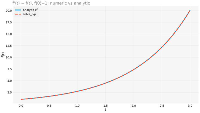
maximum error numeric × analytic: 1.581241804160527e-09With \(f(0) = 1\) fixing the constant (\(C_1 = 1\)), the numerical curve
falls right on top of the analytic curve \(e^t\), with an error on the
order of \(10^{-9}\), a pure artifact of numerical tolerance, not of the
technique. dense_output=True makes it possible to evaluate the solution at
any point of the interval after solving, which is what sol.sol(t_plot)
does here.
But two parameters showed up without explanation, rtol and atol, and they
will reappear in almost every call in this article. It is worth
understanding what they mean before moving on.
rtol and atol: how solve_ivp decides whether a step is good
Every adaptive step-size method needs a criterion to accept or
reject a step. solve_ivp estimates the error made in each step and
compares it with a limit built from the two parameters:
If the error exceeds this limit, the step is rejected and redone with a smaller \(h\); if it stays well below, the integrator allows itself to increase \(h\) on the next step. That is how it chooses the step size on its own.
The two play different roles, which is why both exist:
rtol(relative tolerance) controls the significant digits. Anrtol=1e-6asks, roughly, for 6 correct digits, regardless of whether \(y\) is \(10^{-3}\) or \(10^{8}\).atol(absolute tolerance) is a floor, and it exists for the case where \(y\) passes near zero. There the term \(\texttt{rtol} \times |y|\) also tends to zero, and demanding relative precision on a tiny number would be impossible: the integrator would keep shrinking the step forever.atolsays “below this absolute value, stop worrying”.
The default values are rtol=1e-3 and atol=1e-6, the same for
all methods, and quite loose: they were chosen to be fast, not
precise. The difference is easy to measure, solving the same exponential
both ways:
import numpy as np
from scipy.integrate import solve_ivp


def exponential_field(t, y):
    return y  # f'(t) = f(t)


t_plot = np.linspace(0, 3, 200)
y_analytic = np.exp(t_plot)

sol_default = solve_ivp(exponential_field, [0, 3], [1.0], dense_output=True)
print("error with the defaults:", np.max(np.abs(sol_default.sol(t_plot)[0] - y_analytic)))
error with the defaults: 0.0020342038563727627An error of \(2 \times 10^{-3}\) against the \(1.6 \times 10^{-9}\) from before: a million times larger, for the same ODE and the same interval. Three correct digits are enough to draw a plot, but not to compare against an analytic solution, which is what we will be doing here all the time. That is why the calls in this article almost always tighten both.
“Almost always”: the stiffness comparison, later on, deliberately uses the defaults, because the step counts of each method only make sense if all of them run under the same criterion, and the default is the criterion most people will use in practice.
import matplotlib.pyplot as plt
import numpy as np
from scipy.integrate import solve_ivp


def exponential_field(t, y):
    return y  # f'(t) = f(t)


sol = solve_ivp(exponential_field, [0, 3], [1.0], dense_output=True, rtol=1e-10, atol=1e-12)

t_plot = np.linspace(0, 3, 200)
y_numeric = sol.sol(t_plot)[0]
y_analytic = np.exp(t_plot)

fig, ax = plt.subplots()
ax.plot(t_plot, y_analytic, label=r"analytic $e^t$")
ax.plot(t_plot, y_numeric, "--", label="solve_ivp")
ax.set_xlabel("t")
ax.set_ylabel("f(t)")
ax.legend()
The following plot shows the two curves overlaid:
The Pendulum That the High School Formula Does Not Describe #
Back to the pendulum from the opening: the exact equation of motion, with no approximation at all, is
$$ \theta''(t) + \frac{g}{L}\sin\theta(t) = 0 $$The \(\sin\theta\) term is the problem: it is nonlinear, and it is exactly what prevents a closed-form solution in terms of elementary functions. The exact solution exists, but it is written with elliptic integrals, which are not elementary functions; we will come back to them shortly, to check the period we will measure numerically. The high school simplification assumes a small angle, \(\sin\theta \approx \theta\), which turns the equation into a linear ODE with a closed-form solution in cosine: \(\theta(t) = \theta_0 \cos(\omega t)\), with \(\omega = \sqrt{g/L}\), hence the period formula, \(T = 2\pi/\omega = 2\pi\sqrt{L/g}\).
solve_ivp needs none of these simplifications, but it only
solves first-order systems, and the pendulum equation is second order.
The conversion is mechanical, and it is worth doing explicitly, because it is
the maneuver that repeats for every high-order ODE:
Name each derivative up to one order below the maximum as a new variable:
$$u_1 = \theta, \qquad u_2 = \dot\theta$$Now write the derivative of each one. The first is immediate, by definition; the second comes from the original equation, isolating \(\ddot\theta\):
$$\dot u_1 = u_2, \qquad \dot u_2 = -\frac{g}{L}\sin u_1$$
Done: two first-order equations, each giving the derivative of one
component as a function of both. That is exactly what the function
field(t, y) needs to return, in the order [u1_dot, u2_dot].
The recipe holds in general: an equation of order \(n\) becomes a system of \(n\) first-order equations, with \(n\) initial conditions. A damped oscillator, an RLC circuit, a mass-spring system: all go through here.
Translating to code, \(\theta\) and \(\dot\theta\) become the two
components of y:
import numpy as np
from scipy.integrate import solve_ivp

g = 9.81  # m/s^2
L = 1.0  # m
omega = np.sqrt(g / L)


def nonlinear_pendulum(t, y):
    theta, theta_dot = y
    return [theta_dot, -(g / L) * np.sin(theta)]


def linear_pendulum(t, theta0):
    return theta0 * np.cos(omega * t)


t_span = [0, 6]
t_eval = np.linspace(*t_span, 400)

for theta0_deg in [10, 60]:
    theta0 = np.radians(theta0_deg)
    sol = solve_ivp(nonlinear_pendulum, t_span, [theta0, 0.0], t_eval=t_eval, rtol=1e-8, atol=1e-10)
    diff_max = np.max(np.abs(np.degrees(sol.y[0] - linear_pendulum(t_eval, theta0))))
    print(f"theta0={theta0_deg} degrees: maximum divergence from the linear approximation = {diff_max:.3f} degrees")
theta0=10 degrees: maximum divergence from the linear approximation = 0.330 degrees
theta0=60 degrees: maximum divergence from the linear approximation = 69.384 degreesFor \(10°\), the small-angle approximation is off by less than half a degree, which is why it works so well in textbook problems, which almost always use small angles. For \(60°\), the divergence exceeds \(69°\).
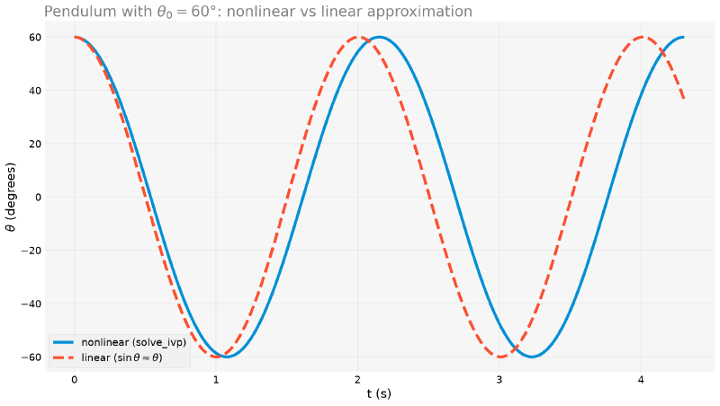
But be careful about what this number means. It is tempting to read “\(69°\) of divergence” as “the approximation gets the shape of the motion wrong”, but that is not it. At \(60°\), the nonlinear solution still looks a lot like a sinusoid; what changes is the period. And since the comparison above runs for \(6\) s, that is, almost three oscillations, a small difference in period accumulates until the two curves are out of phase. The \(69°\) measure accumulated phase drift, not shape error.
Measuring the Real Period #
The hook that opened this article was exactly about this: a pendulum released
from a large angle has a longer period than \(2\pi\sqrt{L/g}\). Time to put
a number on it, and the right tool is the events parameter
of solve_ivp, which stops (or just records) the integration when a
function of the state crosses zero.
Here, the pendulum starts from rest, so the angular velocity \(\dot\theta\) returns to zero exactly at each extreme of the oscillation. Detecting this crossing gives half a period:
import numpy as np
from scipy.integrate import solve_ivp

g = 9.81  # m/s^2
L = 1.0  # m


def nonlinear_pendulum(t, y):
    theta, theta_dot = y
    return [theta_dot, -(g / L) * np.sin(theta)]


def zero_velocity(t, y):
    return y[1]  # theta dot

zero_velocity.direction = 1  # only negative-to-positive crossings

T0 = 2 * np.pi * np.sqrt(L / g)

for theta0_deg in [10, 60, 90, 170]:
    theta0 = np.radians(theta0_deg)
    sol = solve_ivp(nonlinear_pendulum, [1e-9, 20], [theta0, 0.0],
                    events=zero_velocity, rtol=1e-11, atol=1e-13)
    T = 2 * sol.t_events[0][0]
    print(f"theta0={theta0_deg:4d}°  T={T:.4f} s   T/T0={T/T0:.4f}")
theta0= 10° T=2.0099 s T/T0=1.0019
theta0= 60° T=2.1529 s T/T0=1.0732
theta0= 90° T=2.3678 s T/T0=1.1803
theta0= 170° T=4.8935 s T/T0=2.4394Now the hook is paid off, with interpretable numbers. At \(10°\), the real period exceeds the high school formula by \(0.2\%\), invisible in any laboratory experiment. At \(60°\), it is already \(7.3\%\). At \(170°\), almost hanging upward, the pendulum takes more than twice the predicted time.
The exact solution of the pendulum exists, but in terms of a
complete elliptic integral of the first kind, \(K(m)\), which is not an
elementary function, and that is why dsolve does not close it:
scipy.special.ellipk computes \(K\), so we can check the numerical
measurement against the exact value:
import numpy as np
from scipy.integrate import solve_ivp
from scipy.special import ellipk

g = 9.81  # m/s^2
L = 1.0  # m


def nonlinear_pendulum(t, y):
    theta, theta_dot = y
    return [theta_dot, -(g / L) * np.sin(theta)]


def zero_velocity(t, y):
    return y[1]  # theta dot

zero_velocity.direction = 1  # only negative-to-positive crossings

T0 = 2 * np.pi * np.sqrt(L / g)

print(f"{'theta0':>7}  {'numeric T':>11}  {'T/T0':>7}  {'(2/pi)K':>8}  {'difference':>10}")
for theta0_deg in [10, 60, 90, 170]:
    theta0 = np.radians(theta0_deg)
    sol = solve_ivp(nonlinear_pendulum, [1e-9, 20], [theta0, 0.0],
                    events=zero_velocity, rtol=1e-11, atol=1e-13)
    T = 2 * sol.t_events[0][0]
    exact = (2 / np.pi) * ellipk(np.sin(theta0 / 2) ** 2)
    print(f"{theta0_deg:>6}°  {T:>11.5f}  {T/T0:>7.5f}  {exact:>8.5f}  {abs(T/T0 - exact):>10.2e}")
theta0 numeric T T/T0 (2/pi)K difference
10° 2.00989 1.00191 1.00191 9.97e-10
60° 2.15287 1.07318 1.07318 9.96e-10
90° 2.36784 1.18034 1.18034 9.95e-10
170° 4.89352 2.43936 2.43936 9.22e-10Agreement to the ninth decimal place in all four rows, and the residual is the event’s own stopping criterion, not an error of the method.
A convention trap: there are two notations for the elliptic integral in
the literature. Some write \(K(k)\), with the modulus \(k\);
others, \(K(m)\), with the parameter \(m = k^2\). SciPy uses the
second, hence the np.sin(theta0/2) ** 2, with the square. Passing
\(k\) instead of \(m\) raises no error at all, only a silently
wrong answer:
import numpy as np
from scipy.special import ellipk

theta0 = np.radians(60)
print("with m = sin²(θ₀/2), correct:", (2 / np.pi) * ellipk(np.sin(theta0 / 2) ** 2))
print("with k = sin(θ₀/2),  wrong  :", (2 / np.pi) * ellipk(np.sin(theta0 / 2)))
with m = sin²(θ₀/2), correct: 1.0731820071493645
with k = sin(θ₀/2), wrong : 1.1803405990160962Notice the wrong value: \(1.1803\) is exactly the right answer for \(\theta_0 = 90°\). In other words, the mistake returns a perfectly plausible number, the kind that would go unnoticed in a review; that is why the check against the numerical solution, done above, is worth it even when an exact formula exists.
There is also the series approximation that many books give, \(T/T_0 \approx 1 + \theta_0^2/16\). It gives \(1.0019\) at \(10°\) and \(1.0685\) at \(60°\), good in the first two cases. But it predicts \(1.55\) at \(170°\), against the real \(2.44\): an error of \(36\%\). The progressive degradation of this series is, in itself, a good lesson on how far an approximation can be stretched.
Sweeping the amplitude from \(1°\) to \(179°\), the three descriptions line up side by side:
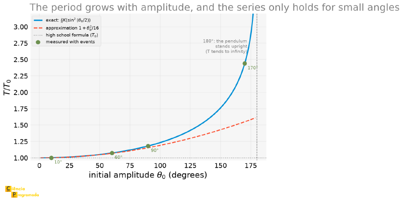
The dotted line at \(1.0\) is what the high school formula predicts: that the period does not depend on the amplitude. It is a good description up to about \(20°\), and that is what makes a pendulum clock possible, as long as it swings little.
And the divergence near \(180°\) has a direct physical meaning: at that amplitude the pendulum reaches the top with zero velocity, in (unstable) equilibrium. It would take an infinite time to complete the oscillation.
Phase Portrait: All the Solutions at Once #
Each call to solve_ivp returns one curve, for one initial
condition. The phase portrait shows the whole set: instead of \(\theta\)
against time, one plots \(\dot\theta\) against \(\theta\), and each
initial condition becomes a closed or open trajectory in this plane.
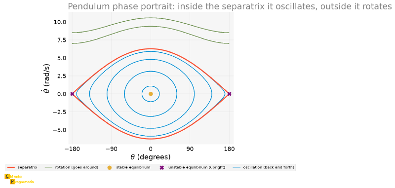
The figure summarizes the entire dynamics in one image:
- The point at the center is the stable equilibrium (pendulum at rest at the bottom). Near it, the curves are almost ellipses: this is the linear regime, the high school one.
- The closed curves are oscillations. The larger the orbit, the larger the amplitude, and, as we just saw, the longer the period.
- The two “X” marks at \(\pm180°\) are the unstable equilibrium: the upright pendulum. They are the same physical point, since \(-180°\) and \(+180°\) coincide.
- The red curve is the separatrix: the trajectory with exactly the energy needed to reach the top, and none to spare. It is the boundary between the two behaviors, and it is what the divergence of the period at \(180°\) corresponds to.
- The open curves, above, are rotations: enough energy to pass the top and keep spinning, always in the same direction.
Notice that none of this is visible in a single solution in time. That is why the phase portrait is the standard tool for understanding nonlinear systems: it shows what can happen, not just what happened with one specific initial condition.
import matplotlib.pyplot as plt
import numpy as np
from scipy.integrate import solve_ivp

g = 9.81  # m/s^2
L = 1.0  # m


def nonlinear_pendulum(t, y):
    theta, theta_dot = y
    return [theta_dot, -(g / L) * np.sin(theta)]


omega = np.sqrt(g / L)


def linear_pendulum(t, theta0):
    return theta0 * np.cos(omega * t)


theta0 = np.radians(60)

# 2 periods of the NONLINEAR pendulum (T = 2.153 s), instead of a fixed 6 s: this way
# the phase lag grows visibly without turning into a tangle of curves
t_span_fig = [0, 2 * 2.1529]
t_eval_fig = np.linspace(*t_span_fig, 400)
sol_pendulum = solve_ivp(nonlinear_pendulum, t_span_fig, [theta0, 0.0], t_eval=t_eval_fig, rtol=1e-8, atol=1e-10)

fig, ax = plt.subplots()
ax.plot(t_eval_fig, np.degrees(sol_pendulum.y[0]), label="nonlinear (solve_ivp)")
ax.plot(t_eval_fig, np.degrees(linear_pendulum(t_eval_fig, theta0)), "--", label=r"linear ($\sin\theta\approx\theta$)")
ax.set_xlabel("t (s)")
ax.set_ylabel(r"$\theta$ (degrees)")
ax.legend()
The following plot makes this visible: the two curves start together, but quickly come apart, because the nonlinear one has a longer period (it oscillates more slowly) than the linear approximation:
Choosing a Method: When the Problem Is Stiff #
solve_ivp accepts several methods via method=, and the right choice can
be the difference between solving in milliseconds or taking much longer
to solve the same equation.
What “Stiffness” Means #
A classic example exposes the problem: \(y^{\prime} = -1000(y - \cos t)\). This equation embeds two very different time scales. The factor \(-1000\) makes any deviation between \(y\) and \(\cos t\) vanish almost instantly: the time scale of this relaxation is \(1/1000 = 0.001\) s. The \(\cos t\) itself, which \(y\) starts to follow closely after this initial transient, varies on a much slower scale (period of \(2\pi \approx 6.3\) s). A system like this, with one component that reacts extremely fast and another that evolves slowly, is called stiff.
The problem is not lack of precision, it is stability: a method like
RK45 (seen next) chooses the step size based on the fastest dynamics
of the system, and keeps needing tiny steps even after that fast dynamics
has already “died” and \(y\) is already evolving smoothly along
with \(\cos t\). If the step exceeds the limit imposed by the fast scale,
the method does not just become imprecise: it diverges numerically (the
solution oscillates and blows up). That is why the integrator is forced to
keep small steps the whole time, even in the “easy” part of the solution,
hence the cost.
Explicit and Implicit Methods, Step by Step #
Every numerical method for ODEs works in the same general way: given the current value, \(y_n\), compute the next one, \(y_{n+1}\), after a step of size \(h\). The difference between an explicit and an implicit method is in how that computation is done.
A method is explicit when it computes \(y_{n+1}\) directly, using only what is already known: the current value and the derivative at it (or at intermediate points already computed from it). The simplest case, the explicit Euler method:
$$y_{n+1} = y_n + h \cdot f(t_n, y_n)$$Everything on the right-hand side is already a known number before the step: just substitute and compute.
A method is implicit when \(y_{n+1}\) appears on both sides of the equation, including inside the very function being integrated. The implicit equivalent of the Euler method above:
$$y_{n+1} = y_n + h \cdot f(t_{n+1}, y_{n+1})$$Since \(y_{n+1}\) is at the same time what we want to find and one of the arguments of \(f\) on the right-hand side, it cannot be isolated in a direct computation: solving this equation normally requires an iterative method (such as Newton’s) at each step.
The Runge-Kutta methods (RK45, RK23, DOP853, seen in the table
below) follow the explicit logic, only combining several
intermediate evaluations of \(f\) in a more precise formula, but always a
direct computation, without having to solve any equation. The extra cost per
step of an implicit method buys stability: its stability region is much
larger, and does not depend on the fast scale of the system the way an
explicit method’s does; that is why it tolerates much larger steps on stiff
problems, like the one in the example above.
import numpy as np
from scipy.integrate import solve_ivp


def stiff(t, y):
    return [-1000 * (y[0] - np.cos(t))]


for method_name in ["RK45", "Radau", "LSODA"]:
    sol = solve_ivp(stiff, [0, 2], [0.0], method=method_name)
    print(f"{method_name:>6}: success={sol.success}  steps={len(sol.t)}  nfev={sol.nfev}")
RK45: success=True steps=611 nfev=4238
Radau: success=True steps=15 nfev=100
LSODA: success=True steps=58 nfev=106RK45 needed \(611\) steps and \(4238\) function evaluations
to solve the same problem that Radau solves in \(15\) steps and
\(100\) evaluations, more than 40 times less work. That is the practical
symptom of stiffness: a number of steps or evaluations much larger than
expected for the default explicit method, on a problem that “does not look”
that complicated.
4,238
RK45
100
Radau
40×
less work
But these counts say how much, not where. Plotting the size of each step along the integration, the mechanism shows up:
import matplotlib.pyplot as plt
import numpy as np
from scipy.integrate import solve_ivp


def stiff(t, y):
    return [-1000 * (y[0] - np.cos(t))]


fig, ax = plt.subplots(figsize=(9, 5.5))
for method_name, color in (("RK45", "C1"), ("Radau", "C0"), ("LSODA", "C3")):
    sol_p = solve_ivp(stiff, [0, 2], [0.0], method=method_name)
    steps = np.diff(sol_p.t)          # the interval between consecutive instants
    ax.semilogy(sol_p.t[1:], steps, "o-", color=color, markersize=3, linewidth=1,
                label=f"{method_name} ({len(sol_p.t)} steps)")
    print(f"{method_name:>6}: median step={np.median(steps):.2e}"
          f"  maximum={steps.max():.2e}")

ax.axhline(1 / 1000, color="C4", linestyle="--", linewidth=1.5,
           label="fast time scale (1/1000 s)")
ax.set_xlabel("t (s)")
ax.set_ylabel("step size h")
ax.legend(fontsize=9)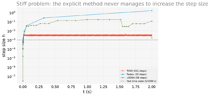
  RK45: median step=3.25e-03  maximum=4.18e-03
 Radau: median step=1.43e-03  maximum=1.67e+00
 LSODA: median step=5.75e-04  maximum=1.75e-01
The maximum step tells the whole story. RK45 never goes past
\(4.2\times10^{-3}\), always in the same order of magnitude as the fast
time scale of the problem (\(1/1000\) s), from start to finish. Radau
reaches \(1.67\), four hundred times larger.
And that is what stiffness means in practice. After the initial transient, the solution is smooth: \(y\) simply follows \(\cos t\), and a large step would deliver the precision without any problem. But the explicit method cannot increase the step: not for lack of precision, but because above a certain \(h\) it becomes unstable and the solution blows up. It remains hostage to a fast dynamics that no longer exists.
What “Order p(q)” Means #
Before the table, it is worth understanding the “order \(p(q)\)” notation that appears in almost every method. It describes an embedded pair of formulas, which run together reusing the same intermediate evaluations of \(f\):
- The solution that actually advances, \(y_{n+1}\), comes from the formula of order \(p\) (the higher one). “Order \(p\)” means that the error accumulated over the integration falls like \(O(h^p)\), the same concept of order already seen in the numerical derivatives article with finite differences (the central one was \(O(h^2)\), the forward/backward, \(O(h)\)): the higher the order, the faster the error falls as \(h\) decreases.
- The formula of order \(q\) (the lower one, in parentheses) does not
advance the solution: it serves only to estimate the step error, comparing
its result with that of the formula of order \(p\). Since the two formulas
share the evaluations of \(f\), this estimate comes at no extra
cost, and it is what allows
solve_ivpto grow or shrink \(h\) on its own along the integration (adaptive step size), without the user having to fix a value.
So “RK45, order 5(4)” reads: it advances with the 5th-order formula and
measures the step error with a 4th-order formula embedded in it.
Quick Guide to Methods #
The following table summarizes the options of solve_ivp, with the full
name behind each acronym and when each one is justified:
| Method | Name behind the acronym | Type | When to use |
|---|---|---|---|
RK45 (default) |
Runge-Kutta, Dormand-Prince pair of formulas, order 5(4) | Explicit | First choice for most non-stiff problems, a good balance between cost and precision |
RK23 |
Runge-Kutta, Bogacki-Shampine pair of formulas, order 3(2) | Explicit | Low precision is acceptable, or the field(t, y) is expensive to evaluate and fewer evaluations per step matter more than the order |
DOP853 |
Dormand-Prince Runge-Kutta, order 8 | Explicit | Smooth, non-stiff problem where high precision is needed, more accurate than RK45, at the cost of more evaluations per step |
Radau |
Implicit Runge-Kutta of the Radau IIA family, order 5(3) | Implicit | Stiff problems that also need high precision |
BDF |
Backward Differentiation Formulas, variable order from 1 to 5 | Implicit | Stiff problems with many variables, robust and efficient on large systems |
LSODA |
Solver from the ODEPACK package (Lawrence Livermore National Laboratory), automatically switching between an Adams-type method (non-stiff) and BDF |
Automatic | When it is not known beforehand whether the problem is stiff, it detects the transition and switches method on its own |
(The full names and the origin of each method come from the SciPy documentation itself, which cites the original papers for each one.)
Without this table as a reference, the reasonable default choice is always
RK45; it is only worth switching when the symptom of stiffness appears
(steps or nfev well above what is expected) or when the precision of
RK45 is not enough for a problem known to be smooth.
Real Applications #
With the basic mechanics and the choice of method established, five applications follow, from the simplest (with a closed-form solution, for validation) to the ones that do not close at all.
Example 1: Logistic population growth
Statement: A population grows according to the logistic model, \(\frac{dP}{dt} = rP\left(1 - \frac{P}{K}\right)\), with growth rate \(r = 0.5\) year\(^{-1}\), carrying capacity \(K=100\), and initial population \(P_0=5\). Solve numerically and compare with the known analytic solution.
Solution: The closed-form solution of this model is \(P(t) = \dfrac{K}{1 + (K/P_0 - 1)e^{-rt}}\):
import numpy as np
from scipy.integrate import solve_ivp

r, K, P0 = 0.5, 100.0, 5.0


def logistic(t, P):
    return [r * P[0] * (1 - P[0] / K)]


def logistic_analytic(t):
    return K / (1 + (K / P0 - 1) * np.exp(-r * t))


t_eval_log = np.linspace(0, 20, 200)
sol_log = solve_ivp(logistic, [0, 20], [P0], t_eval=t_eval_log, rtol=1e-8, atol=1e-10)
error = np.max(np.abs(sol_log.y[0] - logistic_analytic(t_eval_log)))
print("maximum error:", error)
maximum error: 5.216148338149651e-06An error on the order of \(10^{-6}\): the nonlinear ODE is solved numerically without the model having to be linearized or simplified in any way, and the result matches the closed-form formula within the requested tolerance.
Example 2: Lotka-Volterra: predator and prey
Statement: The Lotka-Volterra predator-prey model describes two coupled populations:
$$\frac{dP}{dt} = \alpha P - \beta P Q, \qquad \frac{dQ}{dt} = \delta P Q - \gamma Q$$The prey \(P\) grows on its own (\(\alpha\)) and is eaten (\(\beta PQ\)); the predator \(Q\) dies on its own (\(\gamma\)) and reproduces by eating (\(\delta PQ\)). Solve with \(\alpha=1\), \(\beta=0.02\), \(\delta=0.01\), \(\gamma=0.5\), starting from 40 prey and 9 predators.
Solution: This is the first example in the article with parameters passed
via args, instead of captured from the global scope, which is the
recommended way, and avoids the class of bug in which changing a global
variable silently changes the result of another cell:
import numpy as np
from scipy.integrate import solve_ivp

def lotka_volterra(t, y, alpha, beta, delta, gamma):
    prey, predator = y
    return [alpha * prey - beta * prey * predator,
            delta * prey * predator - gamma * predator]

params = (1.0, 0.02, 0.01, 0.5)   # alpha, beta, delta, gamma
sol_lv = solve_ivp(lotka_volterra, [0, 40], [40.0, 9.0],
                   t_eval=np.linspace(0, 40, 2000),
                   args=params, rtol=1e-10, atol=1e-12)
The system is genuinely nonlinear (the \(PQ\) term couples the two) and has no closed-form solution. But it has a conserved quantity:
$$V = \delta P - \gamma\ln P + \beta Q - \alpha\ln Q$$which serves as a quality test for the integrator, just as mass conservation will in the kinetics example, further on:
import numpy as np
from scipy.integrate import solve_ivp

def lotka_volterra(t, y, alpha, beta, delta, gamma):
    prey, predator = y
    return [alpha * prey - beta * prey * predator,
            delta * prey * predator - gamma * predator]

params = (1.0, 0.02, 0.01, 0.5)   # alpha, beta, delta, gamma
sol_lv = solve_ivp(lotka_volterra, [0, 40], [40.0, 9.0],
                   t_eval=np.linspace(0, 40, 2000),
                   args=params, rtol=1e-10, atol=1e-12)

prey, predator = sol_lv.y
V = 0.01 * prey - 0.5 * np.log(prey) + 0.02 * predator - 1.0 * np.log(predator)
print(f"relative variation of the invariant: {(V.max() - V.min()) / abs(V.mean()):.2e}")
relative variation of the invariant: 7.30e-10The two panels below show the result in time and in the phase plane:
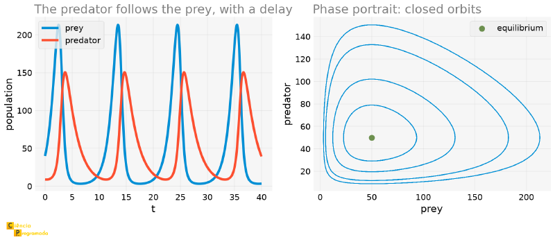
The left panel shows the behavior that gives the model its name. Both populations oscillate, but out of step: the predator only thrives after the prey has thrived, and the predator’s collapse comes after the prey’s collapse.
The right one is the phase portrait, the same tool used on the pendulum: each initial condition generates a closed orbit around the equilibrium at \((50, 50)\), which is where both derivatives vanish (\(P^\ast = \gamma/\delta\), \(Q^\ast = \alpha/\beta\)). A closed orbit means the system returns exactly to the starting point: the oscillations neither damp nor grow, which is a peculiarity of this model, and one of the reasons it is more a caricature than a realistic description of ecosystems.
Example 3: Charging RC circuit
Statement: An uncharged capacitor (\(V(0)=0\)) is connected to a \(5\) V source through a \(1\) k\(\Omega\) resistor and a \(1\) mF capacitor. Find the voltage across the capacitor over time.
Solution: The 1st-order linear ODE \(RC\dfrac{dV}{dt} + V = V_0\) has a known closed-form solution, \(V(t) = V_0(1 - e^{-t/RC})\), one more validation with a closed-form solution before moving on to more complex examples:
import numpy as np
from scipy.integrate import solve_ivp

R, C, V0 = 1e3, 1e-3, 5.0  # ohm, F, V
tau = R * C


def rc_charging(t, V):
    return [(V0 - V[0]) / tau]


t_eval_rc = np.linspace(0, 5 * tau, 200)
sol_rc = solve_ivp(rc_charging, [0, 5 * tau], [0.0], t_eval=t_eval_rc, rtol=1e-8, atol=1e-10)
V_analytic = V0 * (1 - np.exp(-t_eval_rc / tau))
print("maximum error:", np.max(np.abs(sol_rc.y[0] - V_analytic)))
maximum error: 9.250205046384963e-09
Example 4: Falling with quadratic air resistance
Statement: An object of mass \(80\) kg falls from rest, subject to gravity and to an air resistance proportional to the square of the velocity (\(F_{\text{drag}} = -kv^2\), with \(k=0.25\) kg/m, a more realistic model than linear drag at higher velocities). Find the velocity as a function of time.
Solution: The equation of motion is \(m\dfrac{dv}{dt} = mg - kv^2\). The terminal velocity, where \(dv/dt=0\), comes out immediately: \(v_t = \sqrt{mg/k}\).
import numpy as np
from scipy.integrate import solve_ivp

m, g_local, k = 80.0, 9.81, 0.25  # kg, m/s^2, kg/m
v_terminal = np.sqrt(m * g_local / k)


def fall_with_drag(t, v):
    return [g_local - (k / m) * v[0] ** 2]


t_eval_fall = np.linspace(0, 15, 200)
sol_fall = solve_ivp(fall_with_drag, [0, 15], [0.0], t_eval=t_eval_fall,
                     rtol=1e-10, atol=1e-12)
print("terminal velocity:", round(v_terminal, 2), "m/s")
print("velocity at t=15s:", round(sol_fall.y[0][-1], 2), "m/s")
terminal velocity: 56.03 m/s
velocity at t=15s: 55.45 m/sAt 15 s, the object is already at \(98.9\%\) of the terminal velocity, but formally never reaches it, since \(v_t\) is an asymptotic limit, not a value reached in finite time.
And this case still has a closed form, which makes it the third validation among these examples. Separating the variables into \(dv/(1 - v^2/v_t^2) = g\ dt\) and integrating, one arrives at a hyperbolic tangent:
$$v(t) = v_t \tanh\left(\frac{g t}{v_t}\right)$$import numpy as np
from scipy.integrate import solve_ivp
m, g_local, k = 80.0, 9.81, 0.25 # kg, m/s^2, kg/m
v_terminal = np.sqrt(m * g_local / k)
def fall_with_drag(t, v):
return [g_local - (k / m) * v[0] ** 2]
t_eval_fall = np.linspace(0, 15, 200)
sol_fall = solve_ivp(fall_with_drag, [0, 15], [0.0], t_eval=t_eval_fall,
rtol=1e-10, atol=1e-12)
v_analytic = v_terminal * np.tanh(g_local * t_eval_fall / v_terminal)
print("maximum error:", np.max(np.abs(sol_fall.y[0] - v_analytic)))maximum error: 1.00780468414996e-08It matches to the eighth decimal place, pure tolerance residue. It is a classic result of mechanics, and it is good that it appears here: “has quadratic drag” is not a synonym for “does not close”.
The article on orbits and trajectories of this series had already solved a problem of the same family (a projectile under air resistance), but as a transcendental equation for the flight time, with linear drag (\(F_{\text{drag}} = -kmv\), 2D, with a launch angle). Here the physics is different (quadratic drag, vertical component only), but the change of approach is the same lesson: without drag simplified enough to isolate a variable in a closed-form equation, solving the ODE directly in time is the way to go.
Example 5: Chemical kinetics: consecutive reactions
Statement: In a reaction \(A \to B \to C\), with rate constants \(k_1=0.3\) s\(^{-1}\) and \(k_2=0.1\) s\(^{-1}\), starting from \(A_0=1\) mol/L and no \(B\) or \(C\), find the concentrations of the three species over time.
Solution: The system of coupled ODEs is \(\frac{dA}{dt}=-k_1A\), \(\frac{dB}{dt}=k_1A-k_2B\), \(\frac{dC}{dt}=k_2B\), three chained equations, each feeding the next:
import numpy as np
from scipy.integrate import solve_ivp

k1, k2 = 0.3, 0.1  # 1/s
A0 = 1.0


def consecutive_reactions(t, y):
    A, B, C = y
    return [-k1 * A, k1 * A - k2 * B, k2 * B]


t_eval_kin = np.linspace(0, 30, 300)
sol_kin = solve_ivp(
    consecutive_reactions, [0, 30], [A0, 0.0, 0.0], t_eval=t_eval_kin, rtol=1e-8, atol=1e-10
)

A_analytic = A0 * np.exp(-k1 * t_eval_kin)
print("maximum error in A(t):", np.max(np.abs(sol_kin.y[0] - A_analytic)))
print("mass conservation deviation:", np.max(np.abs(sol_kin.y.sum(axis=0) - A0)))
maximum error in A(t): 4.733793357303284e-10
mass conservation deviation: 4.440892098500626e-16Two checks: \(A(t)\) matches the pure exponential (since \(A\) does not depend on \(B\) or \(C\)), and the sum \(A+B+C\) remains equal to \(A_0\) the whole time. That is mass conservation, which no line of code imposed explicitly and which only follows from how the three equations were written.
And we can check more. This system, although coupled, has a closed-form solution, a classic result of chemical kinetics:
$$B(t) = \frac{k_1 A_0}{k_2-k_1}\left(e^{-k_1t}-e^{-k_2t}\right)$$import numpy as np
from scipy.integrate import solve_ivp
k1, k2 = 0.3, 0.1 # 1/s
A0 = 1.0
def consecutive_reactions(t, y):
A, B, C = y
return [-k1 * A, k1 * A - k2 * B, k2 * B]
t_eval_kin = np.linspace(0, 30, 300)
sol_kin = solve_ivp(
consecutive_reactions, [0, 30], [A0, 0.0, 0.0], t_eval=t_eval_kin, rtol=1e-8, atol=1e-10
)
B_analytic = A0 * k1 / (k2 - k1) * (np.exp(-k1 * t_eval_kin) - np.exp(-k2 * t_eval_kin))
print("maximum error in B(t):", np.max(np.abs(sol_kin.y[1] - B_analytic)))maximum error in B(t): 7.066555118839801e-10A third check, and the most demanding of the three: the entire curve of the intermediate, with its characteristic peak, reproduced to the ninth decimal place.
import matplotlib.pyplot as plt
import numpy as np
from scipy.integrate import solve_ivp

k1, k2 = 0.3, 0.1  # 1/s
A0 = 1.0


def consecutive_reactions(t, y):
    A, B, C = y
    return [-k1 * A, k1 * A - k2 * B, k2 * B]


t_eval_kin = np.linspace(0, 30, 300)
sol_kin = solve_ivp(
    consecutive_reactions, [0, 30], [A0, 0.0, 0.0], t_eval=t_eval_kin, rtol=1e-8, atol=1e-10
)

fig, ax = plt.subplots()
for curve, name in zip(sol_kin.y, ["A", "B", "C"]):
    ax.plot(t_eval_kin, curve, label=name)
ax.set_xlabel("t (s)")
ax.set_ylabel("concentration (mol/L)")
ax.legend()
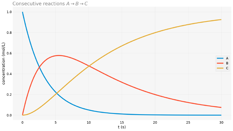
The following plot shows the three concentrations over time:
Where the Closed-Form Formula Really Breaks #
If the system closes, why solve it numerically? Because the formula is fragile in two ways, and both show up early.
First: it blows up when \(k_1 = k_2\). Notice the \(k_2 - k_1\) in the denominator. It is not a physical singularity (two steps with the same rate constant are perfectly reasonable): it is a singularity of the formula. In Python, the result is literally an exception:
import numpy as np

A0 = 1.0
t = np.linspace(0, 30, 300)

k1 = k2 = 0.2
B_analytic = A0 * k1 / (k2 - k1) * (np.exp(-k1 * t) - np.exp(-k2 * t))
ZeroDivisionError: float division by zeroThe correct solution in this case exists, but it has a different functional form, in which the difference of exponentials disappears and a factor \(t\) enters:
$$ B(t) = A_0 k t e^{-kt} $$To get there one has to redo the integration from scratch, or take the limit
\(k_2 \to k_1\) with L’Hôpital. solve_ivp, on the other hand, notices no
difference at all. It is the same field, the same code, and the answer comes
out right:
import numpy as np
from scipy.integrate import solve_ivp

k1 = k2 = 0.2  # the degenerate case
A0 = 1.0


def consecutive_reactions(t, y):
    A, B, C = y
    return [-k1 * A, k1 * A - k2 * B, k2 * B]


t_eval_kin = np.linspace(0, 30, 300)
sol_deg = solve_ivp(consecutive_reactions, [0, 30], [A0, 0.0, 0.0],
                    t_eval=t_eval_kin, rtol=1e-8, atol=1e-10)
print("error against A0*k*t*exp(-k*t):",
      np.max(np.abs(sol_deg.y[1] - A0 * 0.2 * t_eval_kin * np.exp(-0.2 * t_eval_kin))))
error against A0*k*t*exp(-k*t): 8.172407195417009e-10Second: it does not survive a slightly more realistic mechanism. It is enough to make the first step reversible (\(A \rightleftharpoons B \to C\), with a constant \(k_{-1}\) going back) for the system to stop being a cascade and become genuinely coupled:
k1, k_minus1, k2 = 0.3, 0.15, 0.1

def reversible_reactions(t, y):
    A, B, C = y
    return [-k1 * A + k_minus1 * B,
            k1 * A - k_minus1 * B - k2 * B,
            k2 * B]
Now \(A\) depends on \(B\), which depends on \(A\). Solving this by
hand means finding the eigenvalues of a \(3\times3\) matrix (the roots
of a cubic characteristic polynomial) and assembling the solution as a
combination of three exponentials with those exponents. It is possible, it
is ugly, and it vanishes completely as soon as a fourth species or a
second-order step is added (where a closed-form solution does not even
exist). For solve_ivp, the change is three lines.
This is the pattern that repeats throughout this series: the closed form does not disappear all at once, it degrades. First it becomes a special case that needs separate handling, then an expression nobody wants to write, then it no longer exists. The numerical method goes through all three stages without changing code, and that is why it is worth having the analytic validation while it exists: it is what gives confidence to use the method when it runs out.
The numerical derivatives article estimated the rate of a 1st-order kinetics from measured concentration data, with no model at all. Here the logic is inverted: starting from the model (the constants \(k_1\), \(k_2\), and the two-step mechanism), the ODE generates the concentration over time, including the characteristic peak of the intermediate \(B\), at \(t = \ln(k_1/k_2)/(k_1-k_2) \approx 5.49\) s, which a pure 1st-order kinetics would never produce.
Points of Attention #
The same pendulum ODE, with different initial conditions (\(10°\), \(60°\), or \(170°\), all starting from rest), gives curves with different periods: 2.01 s, 2.15 s, and 4.89 s. This is a peculiarity of nonlinear equations worth highlighting: in a linear oscillator, the period does not depend on the amplitude (which is what makes a pendulum clock possible, as long as it swings little). As soon as \(\sin\theta\) enters without approximation, this independence ends.
solve_ivp always solves one specific IVP: change the initial condition,
and the whole curve changes. This is quite different from the general
family that symbolic dsolve returns, with the constant \(C_1\) left
open: there, “the solution” is a family; here, it is always one curve.
atol, rtol) silently affects the result
Solving the \(60°\) pendulum twice, with different tolerances:
import numpy as np
from scipy.integrate import solve_ivp

g = 9.81  # m/s^2
L = 1.0  # m


def nonlinear_pendulum(t, y):
    theta, theta_dot = y
    return [theta_dot, -(g / L) * np.sin(theta)]


t_span = [0, 6]
t_eval = np.linspace(*t_span, 400)
theta0 = np.radians(60)

sol_tight = solve_ivp(nonlinear_pendulum, t_span, [theta0, 0.0], t_eval=t_eval, rtol=1e-10, atol=1e-12)
sol_loose = solve_ivp(nonlinear_pendulum, t_span, [theta0, 0.0], t_eval=t_eval, rtol=1e-2, atol=1e-2)
diff = np.max(np.abs(np.degrees(sol_tight.y[0] - sol_loose.y[0])))
print("maximum divergence:", round(diff, 3), "degrees")
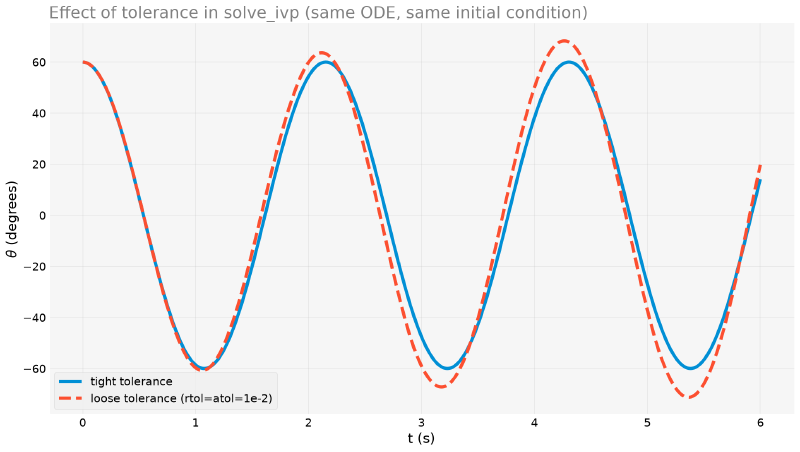
maximum divergence: 12.628 degreesMore than \(12°\) of difference between two “apparently identical”
solve_ivp calls: same ODE, same initial condition, only the tolerance
changed.
Notice where the default sits in this comparison: rtol=1e-3 is between
the two, ten times tighter than the loose version and ten million times
looser than the tight one. In other words, accepting the default without
thinking is not a neutral choice: it is a choice, and on this problem it
would still leave error visible to the naked eye after a few oscillations.
The practical recipe is simple: solve twice, with different tolerances, and compare. If the two curves coincide, the looser tolerance was already enough. If they do not, tighten until they do. It is the equivalent, for ODEs, of the “check the residual” that the article on roots, at the start of this series, recommended.
import matplotlib.pyplot as plt
import numpy as np
from scipy.integrate import solve_ivp

g = 9.81  # m/s^2
L = 1.0  # m


def nonlinear_pendulum(t, y):
    theta, theta_dot = y
    return [theta_dot, -(g / L) * np.sin(theta)]


t_span = [0, 6]
t_eval = np.linspace(*t_span, 400)
theta0 = np.radians(60)

sol_tight = solve_ivp(nonlinear_pendulum, t_span, [theta0, 0.0], t_eval=t_eval, rtol=1e-10, atol=1e-12)
sol_loose = solve_ivp(nonlinear_pendulum, t_span, [theta0, 0.0], t_eval=t_eval, rtol=1e-2, atol=1e-2)

fig, ax = plt.subplots()
ax.plot(t_eval, np.degrees(sol_tight.y[0]), label="tight tolerance")
ax.plot(t_eval, np.degrees(sol_loose.y[0]), "--", label="loose tolerance (rtol=atol=1e-2)")
ax.set_xlabel("t (s)")
ax.set_ylabel(r"$\theta$ (degrees)")
ax.legend()
The two curves start together and come apart over time, the same kind of progressive divergence already seen between the nonlinear pendulum and its linear approximation, now caused only by numerical tolerance:
Summary Table #
| Tool / concept | Use | Note |
|---|---|---|
dsolve (SymPy) |
General symbolic solution, with open constants | Only works when a closed form exists |
solve_ivp(field, t_span, y0) |
Numerical solution of a specific IVP | field(t, y) returns the derivative of each component of y |
dense_output=True |
Allows evaluating the solution at any point after solving | Uses sol.sol(t) |
| Explicit method | Computes \(y_{n+1}\) directly, using only known values | Simple computation, no equation to solve, but unstable on stiff problems with a large step |
| Implicit method | \(y_{n+1}\) appears on both sides of the equation | More expensive per step (requires solving the equation), but much more stable |
| Order \(p(q)\) | Embedded pair: advances with the formula of order \(p\), estimates the error with the one of order \(q\) | Basis of the adaptive step size, error estimated without extra evaluations |
method="RK45" (default) |
Explicit Runge-Kutta | Fast in most cases; inefficient on stiff problems |
method="Radau" / "BDF" |
Implicit methods | Choice for stiff systems |
method="LSODA" |
Detects stiffness automatically | Switches method on its own |
| Symptom of stiffness | Number of steps/evaluations far above what is expected | Compare len(sol.t) or sol.nfev across methods |
| Initial condition | Determines which specific curve is obtained | Different from the general family of dsolve |
Tolerance (rtol, atol) |
Controls precision vs. computational cost | Two solutions with different tolerances can diverge visibly |
Next Steps #
This article covered how to solve a differential equation when there is no
closed-form solution, but always starting from an already written model, with
the equations and parameters known beforehand. A sibling problem
remains: what if what we want is not to solve the ODE, but to find the
best parameters for a model, or the minimum (or maximum) point
of a function with no closed-form formula for its derivative? In the
next article,
scipy.optimize tackles exactly this problem, and, later in the
series, in an article on optimization applications, the very differential
equation solved here comes back as part of the model to be
optimized.


