

In 1959, the English mathematician James H. Wilkinson was investigating why root-finding algorithms, considered correct on paper, behaved badly on the first digital computers. To test a hypothesis, he built a deliberately harmless polynomial, now known as Wilkinson’s polynomial:
$$ (x-1)(x-2)(x-3)\cdots(x-20) $$Degree 20, twenty integer roots, from 1 to 20, all well separated from one another. There is no more “polite” polynomial than this one, or so it seemed. Wilkinson expanded the product into its 21 coefficients and fed them to a numerical algorithm.
And those coefficients are monstrous. The constant term is \(20!\), a
19-digit integer; the largest of all, the coefficient of \(x^2\), exceeds
\(1.38 \times 10^{19}\). Keep that number in mind: the largest integer
that a float64 represents without any error is \(2^{53} \approx 9 \times
10^{15}\), about a thousand times smaller. In other words, a good part of
these coefficients does not even fit exactly in a float: the damage starts
before any algorithm runs.
The result left Wilkinson perplexed enough that, decades later, he described that moment as “the most traumatic experience in my career as a numerical analyst”.
What happened? That is what we will reconstruct in this article, with real code, after learning to handle polynomials as objects in NumPy.
Why Do Polynomials as Objects Matter? #
- Numerical analysis and scientific computing: any method that approximates a function by a polynomial (interpolation, quadrature, differential equation solvers) depends on knowing that high-degree polynomials can amplify small errors dramatically, the very problem Wilkinson discovered.
- Control engineering: the stability of a linear system (electrical, mechanical) usually boils down to where the roots of a characteristic polynomial are. Knowing that these roots can be sensitive to measurement errors in the coefficients is a practical concern.
- Computer graphics: Bézier curves and splines, used in most vector editors and game engines, are polynomials handled numerically: evaluated, differentiated, and fitted thousands of times per second.
- Signal processing: digital filters are described by a ratio of polynomials (the transfer function); the location of the roots of the denominator polynomial (the poles) determines whether the filter is stable.
SymPy Polynomials, Revisited in NumPy #
In the article Polynomials with SymPy
we saw the Poly class, which treats a polynomial as an object (with
methods for coefficients, degree, roots, derivative and integral) instead of
a mere symbolic expression. NumPy has its equivalent:
numpy.polynomial.Polynomial. The essential difference is that here the
coefficients are not exact symbols but floating-point numbers (float64),
which seems like an irrelevant detail and, as we will see at the end of this
article, is not.
Example 1: Recreating a polynomial from the SymPy article
Statement: The SymPy article used \(Q(x) = x^2 - 25\) as a recurring
example. Build the same polynomial with numpy.polynomial.Polynomial and
compare the coefficients with SymPy’s.
Solution: Polynomial takes the coefficients in increasing order of
degree, that is, the first element is the constant term, not the one of
highest degree (more on this in the next section):
import sympy
from numpy.polynomial import Polynomial

x = sympy.Symbol("x")
Q_sym = sympy.Poly(x**2 - 25, x)
Q_np = Polynomial([-25, 0, 1])  # -25 + 0x + 1x^2

print("SymPy all_coeffs (descending):", Q_sym.all_coeffs())
print("NumPy .coef (ascending):", Q_np.coef)
SymPy all_coeffs (descending): [1, 0, -25]
NumPy .coef (ascending): [-25. 0. 1.]Same polynomial, two opposite orders for storing the coefficients.
Trap No. 1: Coefficient Order #
NumPy actually has two ways of representing a polynomial, and neither of them agrees with SymPy:
| Representation | Coefficient order | Example for \(Q(x)=x^2-25\) |
|---|---|---|
numpy.poly1d (legacy) |
Descending | [1, 0, -25] |
numpy.polynomial.Polynomial (modern) |
Ascending | [-25, 0, 1] |
sympy.Poly.all_coeffs() |
Descending | [1, 0, -25] |
poly1d is NumPy’s old API: it still works, but it is considered legacy;
the documentation recommends Polynomial for new code. The risk lies in
mixing them without noticing, since no convention is the “right” one:
passing the coefficient list the wrong way to the wrong class raises no
error at all and silently returns a different polynomial.
As a check, the two NumPy constructors arrive at the same roots for the same \(Q(x)\), despite the opposite coefficient order:
import numpy as np
from numpy.polynomial import Polynomial

Q_np = Polynomial([-25, 0, 1])  # -25 + 0x + 1x^2
p_legacy = np.poly1d([1, 0, -25])  # descending
print("poly1d.roots:", p_legacy.roots)
print("Polynomial.roots():", Q_np.roots())
poly1d.roots: [-5. 5.]
Polynomial.roots(): [-5. 5.]Roots, Including Complex Ones #
Example 2: Roots of a degree-3 polynomial
Statement: The SymPy article also used \(A(x) = x^3 + 2x + 3\), which
has one real root and two complex ones. Find the roots with
Polynomial.roots().
Solution:
from numpy.polynomial import Polynomial

A_np = Polynomial([3, 2, 0, 1])  # 3 + 2x + 0x^2 + 1x^3
print(A_np.roots())
[-1. +0.j 0.5-1.6583124j 0.5+1.6583124j]SymPy needed two separate methods for this (all_roots() for all the roots,
real_roots() for the real ones only), because, for SymPy, a real root and
a complex root are mathematically distinct objects. Polynomial.roots()
makes no such distinction and returns a single numeric array, real when all
the roots are real and complex (with zero imaginary part in the real roots)
when there is any complex root, because for NumPy a polynomial is, above
all, an array of numeric coefficients, the same philosophy as numpy.roots
already used in
Solving Equations Numerically with SciPy,
now applied to polynomials as objects.
Derivative, Integral and Division #
Example 3: Derivative, integral and division of polynomials
Statement: Compute the derivative of \(Q(x)=x^2-25\) at \(x=2\), the integral of \(Q(x)\) at \(x=1\) (integration constant zero), and the quotient and remainder of dividing \(A(x)=x^3+2x+3\) by \(Q(x)\).
Solution:
from numpy.polynomial import Polynomial

Q_np = Polynomial([-25, 0, 1])   # -25 + x^2
A_np = Polynomial([3, 2, 0, 1])  # 3 + 2x + x^3

print("Q'(2):", Q_np.deriv()(2))
print("integral of Q up to 1:", Q_np.integ()(1))

quotient, remainder = divmod(A_np, Q_np)
print("quotient:", quotient)
print("remainder:", remainder)
Q'(2): 4.0
integral of Q up to 1: -24.666666666666668
quotient: 0.0 + 1.0·x
remainder: 3.0 + 27.0·xThe same results as in the SymPy article: \(Q^{\prime}(2)=4\), \(\int_0^1 Q dx = -\frac{74}{3} \approx -24.667\), and dividing \(A\) by \(Q\) gives quotient \(x\) and remainder \(27x+3\). As always in a division, \(Q \cdot \text{quotient} + \text{remainder} = A\).
divmod here is Python’s built-in divmod
divmod(A_np, Q_np) is not a NumPy function: it is the language’s
built-in divmod(). It works because Polynomial implements the special
method __divmod__ (along with +, -, *, //, %, **, ==),
returning two new Polynomial objects (quotient and remainder). The
NumPy documentation on the polynomial convenience
classes
explicitly lists these overloaded operators.
Where Did SymPy’s Exactness Go? #
In the SymPy introduction article,
the integer coefficients of a polynomial were exact: sympy.Integer, with
no rounding at all. Here, Q_np.coef is already numpy.float64 from the
moment of construction. For a low-degree polynomial like \(Q\) or \(A\),
this changes nothing visible. But as the degree grows, the difference
between “exact” and “floating point” stops being cosmetic; it is time to go
back to the polynomial that opened this article.
Back to Wilkinson’s Polynomial #
What Wilkinson discovered has a name, and it is worth defining it before reproducing the experiment:
A numerical problem is ill-conditioned when a tiny change in the input data produces a disproportionately large change in the answer, even using a perfectly correct algorithm. It is not a code bug; it is a property of the problem itself.
Time to reproduce Wilkinson’s experiment, step by step.
Step 1: the exact coefficients, with SymPy #
First, we expand \((x-1)(x-2)\cdots(x-20)\) symbolically (the same tool used in the previous articles of the series) to get the 21 coefficients with no rounding error:
import sympy

x = sympy.Symbol("x")
wilkinson_expr = sympy.prod([x - k for k in range(1, 21)])
wilkinson_poly_sym = sympy.Poly(wilkinson_expr, x)

coefs_desc = wilkinson_poly_sym.all_coeffs()  # descending, exact integers
print("coefficient of x^19:", coefs_desc[1])
print("constant term (20!):", coefs_desc[-1])
coefficient of x^19: -210
constant term (20!): 2432902008176640000Notice the size of these numbers: the constant term is already \(20!\), a 19-digit integer. All 21 coefficients, at this point, are still exact.
The following figure shows the magnitude of all of them, on a logarithmic
scale, with the line of the largest integer that a float64 stores without
any error:
import matplotlib.pyplot as plt
import numpy as np
import sympy

x = sympy.Symbol("x")
wilkinson_expr = sympy.prod([x - k for k in range(1, 21)])
coefs_desc = sympy.Poly(wilkinson_expr, x).all_coeffs()  # descending, exact integers
magnitudes = [abs(int(c)) for c in reversed(coefs_desc)]  # ascending, still exact

degrees = np.arange(21)
fig, ax = plt.subplots(figsize=(8, 5))
ax.bar(degrees, [float(m) for m in magnitudes], color="C0")
ax.axhline(2.0**53, color="C1", linestyle="--", linewidth=2,
           label=r"$2^{53}$: largest exact integer in float64")
ax.set_yscale("log")
ax.set_xlabel("degree of the term")
ax.set_ylabel(r"$|$coefficient$|$")
ax.legend()

print(f"{sum(m > 2**53 for m in magnitudes)} of the 21 coefficients exceed 2^53")
10 of the 21 coefficients exceed 2^53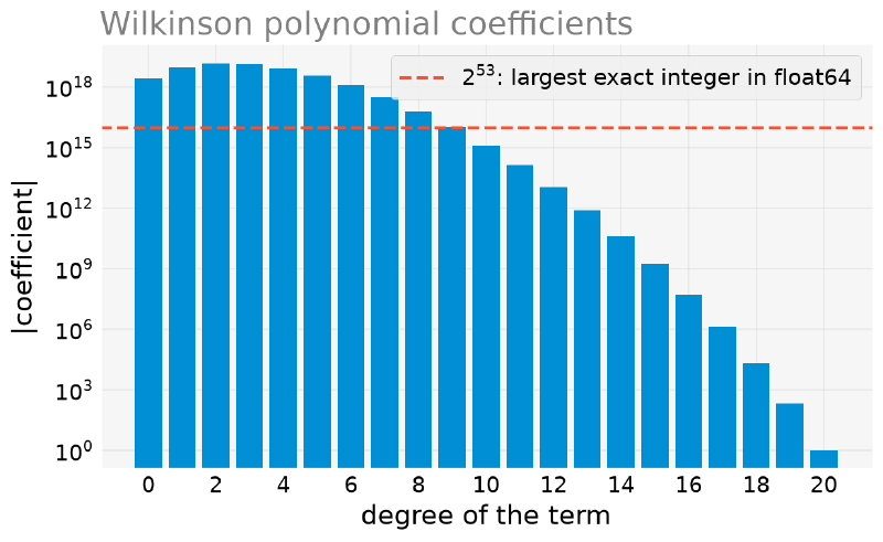
Ten of the twenty-one coefficients are above the line. Each of them already
reaches float64 with error, not because of any algorithm, but because the
format cannot hold the number.
Step 2: converting to float64, and error already appears
#
Now comes the part that any NumPy Polynomial requires: converting these
exact integers to float64. That alone is already a perturbation:
import sympy
from numpy.polynomial import Polynomial

x = sympy.Symbol("x")
wilkinson_expr = sympy.prod([x - k for k in range(1, 21)])
coefs_desc = sympy.Poly(wilkinson_expr, x).all_coeffs()  # descending, exact integers

wilkinson_coefs = [float(c) for c in reversed(coefs_desc)]
W = Polynomial(wilkinson_coefs)
With the polynomial built, we compute the roots and compare them with the expected values (the integers from 1 to 20):
import numpy as np
import sympy
from numpy.polynomial import Polynomial

x = sympy.Symbol("x")
wilkinson_expr = sympy.prod([x - k for k in range(1, 21)])
coefs_desc = sympy.Poly(wilkinson_expr, x).all_coeffs()  # descending, exact integers
wilkinson_coefs = [float(c) for c in reversed(coefs_desc)]
W = Polynomial(wilkinson_coefs)

roots = W.roots()
max_error = np.max(np.abs(np.sort(roots.real) - np.arange(1, 21)))
print(f"maximum error, with no deliberate perturbation: {max_error:.4f}")
print("roots computed for the expected values 14 and 15:")
print(np.sort_complex(roots)[13:15])
maximum error, with no deliberate perturbation: 0.5185
roots computed for the expected values 14 and 15:
[14.518475-0.20853241j 14.518475+0.20853241j]It is worth rereading that output carefully, because it is more dramatic than it looks: the roots stopped being real. Where two integers should be, \(14\) and \(15\), there is a pair of complex conjugates, \(14.518 \pm 0.209i\).
And none of this was perturbed on purpose. The only “insult” to the
polynomial was converting its exact integer coefficients to float64, which
is unavoidable, since it is what any NumPy Polynomial requires.
.roots().real
It is tempting to write W.roots().real to “clean up” the result. But
.real silently discards the imaginary part: the conjugate pair above
becomes two identical values, \(14.518\) and \(14.518\), and the reader
concludes that the roots merely “collided”. The most important
information, that they left the real axis, vanishes without warning.
When you want only the truly real roots, filter instead of truncating:
roots[np.abs(roots.imag) < tol].real.
To measure how fragile this is, here is an experiment that perturbs nothing
on purpose: building the same polynomial by two different paths. One is the
one we just used (expand with SymPy, convert to float64); the other is
Polynomial.fromroots, which multiplies the factors directly in floating
point.
import numpy as np
import sympy
from numpy.polynomial import Polynomial

x = sympy.Symbol("x")
wilkinson_expr = sympy.prod([x - k for k in range(1, 21)])
coefs_desc = sympy.Poly(wilkinson_expr, x).all_coeffs()  # descending, exact integers
wilkinson_coefs = [float(c) for c in reversed(coefs_desc)]
W = Polynomial(wilkinson_coefs)

W_via_sympy = W
W_via_fromroots = Polynomial.fromroots(np.arange(1, 21))

print("are the coefficients equal?", np.allclose(W_via_sympy.coef, W_via_fromroots.coef))
print("largest relative difference:",
      np.max(np.abs(W_via_sympy.coef - W_via_fromroots.coef) /
             np.maximum(np.abs(W_via_sympy.coef), 1)))
print()
print("roots 14/15, via SymPy    :", np.sort_complex(W_via_sympy.roots())[13:15])
print("roots 14/15, via fromroots:", np.sort_complex(W_via_fromroots.roots())[13:15])
are the coefficients equal? True
largest relative difference: 1.5911824568028567e-16
roots 14/15, via SymPy : [14.518475-0.20853241j 14.518475+0.20853241j]
roots 14/15, via fromroots: [14.51819694-0.20459637j 14.51819694+0.20459637j]Read these numbers slowly. The coefficients of the two polynomials differ,
at most, by \(1.6\times10^{-16}\) relative, that is, by a single bit in
the last digit of the float64. It is the smallest difference that exists
between two different numbers in this representation; any smaller and they
would be identical.
And the roots differ in the fourth decimal place: the imaginary part goes from \(0.2085\) to \(0.2046\), almost \(2\%\).
Neither path is wrong, and no algorithm failed. Simply, in float64, there
is no single answer to the question “what are the roots of this
polynomial”: the question is too sensitive for the format in which it was
asked. It is this phenomenon that has a name, and it is what we will
perturb on purpose next, to measure it.
Step 3: Wilkinson’s classic perturbation #
Now, deliberately, we decrease a single coefficient, the one of \(x^{19}\), which is exactly \(-210\), by just \(2^{-23} \approx 1.19\times10^{-7}\). This exponent is the machine epsilon of single precision, the 32-bit format with 23 significand bits that we detailed in the article on IEEE 754. It is an error smaller than that of any reasonable experimental measurement.
import numpy as np
import sympy
from numpy.polynomial import Polynomial

x = sympy.Symbol("x")
wilkinson_expr = sympy.prod([x - k for k in range(1, 21)])
coefs_desc = sympy.Poly(wilkinson_expr, x).all_coeffs()  # descending, exact integers
wilkinson_coefs = [float(c) for c in reversed(coefs_desc)]
W = Polynomial(wilkinson_coefs)

perturbed_coefs = np.array(wilkinson_coefs, dtype=float)
perturbed_coefs[19] -= 2**-23
W_perturbed = Polynomial(perturbed_coefs)
Step 4: what happened to the roots #
With the perturbed polynomial built, we recompute the roots and compare them with the original ones:
import numpy as np
import sympy
from numpy.polynomial import Polynomial

x = sympy.Symbol("x")
wilkinson_expr = sympy.prod([x - k for k in range(1, 21)])
coefs_desc = sympy.Poly(wilkinson_expr, x).all_coeffs()  # descending, exact integers
wilkinson_coefs = [float(c) for c in reversed(coefs_desc)]
W = Polynomial(wilkinson_coefs)

perturbed_coefs = np.array(wilkinson_coefs, dtype=float)
perturbed_coefs[19] -= 2**-23
W_perturbed = Polynomial(perturbed_coefs)

perturbed_roots = W_perturbed.roots()
max_imag_part = np.max(np.abs(perturbed_roots.imag))
real_roots = perturbed_roots[np.abs(perturbed_roots.imag) < 1e-6].real
root_that_was_20 = real_roots[np.argmin(np.abs(real_roots - 20))]

print(f"largest imaginary part that appeared: {max_imag_part:.4f}")
print(f"root that was 20 became: {root_that_was_20:.4f}")
largest imaginary part that appeared: 2.8127
root that was 20 became: 20.8469Ten of the twenty roots stop being real. The root that was exactly 20 rises to \(\approx 20.85\), a deviation of \(4.2\%\) caused by a perturbation of \(10^{-7}\) in a single coefficient out of twenty.
Step 5: visualizing the scattering of the roots #
The following plot puts side by side the original roots, all real (circles, aligned on the x axis), and the perturbed roots, scattered across the complex plane (x):
import matplotlib.pyplot as plt
import numpy as np
import sympy
from numpy.polynomial import Polynomial

x = sympy.Symbol("x")
wilkinson_expr = sympy.prod([x - k for k in range(1, 21)])
coefs_desc = sympy.Poly(wilkinson_expr, x).all_coeffs()  # descending, exact integers
wilkinson_coefs = [float(c) for c in reversed(coefs_desc)]
W = Polynomial(wilkinson_coefs)

perturbed_coefs = np.array(wilkinson_coefs, dtype=float)
perturbed_coefs[19] -= 2**-23
perturbed_roots = Polynomial(perturbed_coefs).roots()

fig, ax = plt.subplots(figsize=(8, 7))
ax.scatter(
    np.arange(1, 21), np.zeros(20),
    label="theoretical roots (integers 1 to 20)", zorder=3, s=60,
)
ax.scatter(
    perturbed_roots.real, perturbed_roots.imag,
    marker="x", label="roots after perturbing 1 coefficient by $2^{-23}$",
    zorder=3, s=60,
)
ax.axhline(0, color="black", linewidth=0.8, zorder=1)
ax.set_xlabel("Real part")
ax.set_ylabel("Imaginary part")
ax.set_title("Sensitivity of the Wilkinson polynomial roots", pad=12)
ax.legend(loc="upper center", bbox_to_anchor=(0.5, -0.12), ncol=1)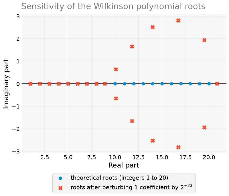
This is what Wilkinson saw in 1959, and the reason his reaction was not an exaggeration.
Why This Happens #
So far the article has shown that it happens. The why is missing, and it fits in a formula.
Perturb the coefficient \(a_k\) by a small amount \(\delta\). Each root \(x_j\) shifts, to first order, by:
$$ \frac{\partial x_j}{\partial a_k} = -\frac{x_j^{k}}{p'(x_j)} $$The derivation is short: if \(p(x_j) = 0\) and we perturb \(a_k\), the new root satisfies \(p(x_j + \Delta) + \delta (x_j+\Delta)^k = 0\). Expanding in a Taylor series and keeping the first order, \(p^{\prime}(x_j)\Delta + \delta x_j^k \approx 0\), which gives the ratio above.
This fraction explains everything, because its two pieces pull in opposite directions as \(j\) grows:
- The numerator \(x_j^{19}\) explodes. For \(x_1 = 1\) it is 1; for \(x_{20} = 20\) it is \(5.2 \times 10^{24}\).
- The denominator \(p^{\prime}(x_j)\) plummets in the middle. Since \(p^{\prime}(x_j) = \prod_{i \neq j}(x_j - x_i)\), it is the product of the 19 distances from \(x_j\) to the other roots. At the ends (\(j=1\) or \(j=20\)) this product is \(19! \approx 10^{17}\), enormous. In the middle (\(j \approx 10\)), half of the differences are small and the product drops to \(10^{12}\).
import sympy
from numpy.polynomial import Polynomial

x = sympy.Symbol("x")
wilkinson_expr = sympy.prod([x - k for k in range(1, 21)])
coefs_desc = sympy.Poly(wilkinson_expr, x).all_coeffs()  # descending, exact integers
wilkinson_coefs = [float(c) for c in reversed(coefs_desc)]
W = Polynomial(wilkinson_coefs)

dW = W.deriv()
print(f"{'j':>3} {'|p_prime(x_j)|':>15} {'x_j^19':>12} {'sensitivity':>15}")
for j in (1, 2, 5, 10, 16, 20):
    xj = float(j)
    print(f"{j:>3} {abs(dW(xj)):>15.2e} {xj**19:>12.2e} {abs(xj**19 / dW(xj)):>15.2e}")
j |p_prime(x_j)| x_j^19 sensitivity
1 1.22e+17 1.00e+00 8.22e-18
2 6.40e+15 5.24e+05 8.19e-11
5 3.14e+13 1.91e+13 6.08e-01
10 1.32e+12 1.00e+19 7.60e+06
16 3.14e+13 7.56e+22 2.41e+09
20 1.22e+17 5.24e+24 4.31e+07The last column varies over 27 orders of magnitude. The root \(x_1 = 1\) is essentially immune (\(8.2 \times 10^{-18}\)); the root \(x_{16}\) is \(2.4 \times 10^{9}\) times more sensitive than the applied perturbation.
The following figure shows that whole column, one bar per root:
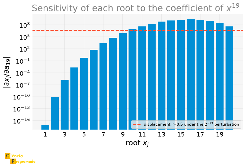
Compare this figure with the result of the experiment: the roots that
survived intact are the small ones, and the ones that became complex pairs
are those from the middle up. The figure predicted which ones would break,
before running roots().
The distinction is the moral of the article. numpy.roots computes the
eigenvalues of the companion matrix with a norm-wise stable algorithm
(backward stable): the result it returns is the exact answer to a
problem very close to the one you passed. It does not err: it answers
accurately a question slightly different from yours.
For well-conditioned problems, that is enough: the exact answer to a nearby problem is a nearby answer. For Wilkinson’s polynomial, it is not enough, because “close in the coefficients” and “close in the roots” stop being the same thing. Changing the algorithm would not help; the problem is in the question, not in who answers it.
It Is Not Just Proximity: Multiplicity Too #
It might seem that the problem is having roots that are “too close”. The opposite extreme shows that it is not:
import numpy as np
from numpy.polynomial import Polynomial

P_mult = Polynomial.fromroots(np.ones(20))   # (x-1)^20
mult_roots = P_mult.roots()
print(f"radius of the scatter around 1: {np.max(np.abs(mult_roots - 1)):.4f}")
print("how many stopped being real:", int((np.abs(mult_roots.imag) > 1e-8).sum()))
radius of the scatter around 1: 0.4352
how many stopped being real: 18\((x-1)^{20}\) has one root, repeated 20 times. roots() returns 20
values scattered on a circle of radius \(0.44\) around 1, and 18 of them
are not even real. It makes sense by the same formula: at a multiple root,
\(p^{\prime}(x_j) = 0\) exactly, and the sensitivity is infinite.
The Practical Lesson #
High-degree roots seem impossible to tame, but the formula suggests the opposite. It points to the culprit, and the culprit is avoidable:
The loss happens at the moment the factors \((x-1)(x-2)\cdots\) become a list of coefficients. Before that, the roots were written in plain sight. Practical rules:
- Keep the factored form whenever it exists.
Polynomial.fromrootsandroots()are inverse operations, but the forward path loses information. - Prefer another basis. The power basis \(1, x, x^2, \ldots\) is terrible on intervals far from the origin. The next article shows that the same polynomial, written in the Chebyshev basis with the domain mapped to \([1, 20]\), becomes millions of times less sensitive.
- If the problem comes from a matrix (eigenvalues, system stability), solve the matrix directly instead of building and solving the characteristic polynomial. The path through the polynomial destroys conditioning for free.
In other words: Wilkinson’s ill-conditioning is not a property of the set of roots \(\{1, \ldots, 20\}\). It is a property of representing it as a list of coefficients in the power basis.
Summary Table #
| Operation | Syntax | Note |
|---|---|---|
| Construction | Polynomial([c0, c1, ..., cn]) |
Ascending order of degree |
| Construction (legacy) | numpy.poly1d([cn, ..., c1, c0]) |
Descending order, avoid in new code |
| Roots | .roots() |
Real array if all roots are real; complex if there is any complex root |
| Derivative | .deriv() |
Returns another Polynomial |
| Integral | .integ() |
Integration constant zero by default |
| Division | divmod(A, B) |
Returns (quotient, remainder) |
| Exact coefficients | Does not exist | Every coefficient is float64; ill-conditioned at high degree (Wilkinson) |
Next Steps #
This article covered polynomials as objects we already knew, built from
coefficients or roots we had in advance. But most real-world data does not
come with a polynomial attached: it comes as a cloud of noisy experimental
points, and it is up to us to find the polynomial that best describes those
points. SymPy does not do that: there is no symbolic regression. In the
next article,
we use Polynomial.fit() to fit curves to real data from chemistry,
physics and engineering, and we see why a higher degree is not always a
better fit: Runge’s phenomenon, a sort of cousin of Wilkinson’s
ill-conditioning, but for interpolation instead of roots.


