

In 1705, the English astronomer Edmond Halley cross-checked records of comets observed in 1531, 1607, and 1682 and reached a bold conclusion: the three could be the same object, returning to the Sun every 76 years or so. Using Kepler’s laws (published almost a century earlier) and the mechanics newly formalized by Newton, Halley computed the orbit and predicted the comet’s return for 1758. He did not live to check: he died in 1742. But the comet came back at the end of 1758, sixteen years later, and took the name of the man who got the prediction right (see the entry Halley’s Comet).
Halley’s prediction was for 1758, with no month or day: he knew that Jupiter and Saturn would perturb the orbit, but he had no way to calculate by how much. The ones who did that calculation were three French astronomers, between 1757 and November 1758: Alexis Clairaut, Jérôme Lalande, and Nicole-Reine Lepaute, who spent months splitting endless intermediate arithmetic sums among themselves to integrate, step by step, the effect of the two giant planets. They arrived at April 13, 1759, with a margin of one month; the actual perihelion was on March 13.
It is one of the great collective numerical calculations of the 18th century, done by hand, in parallel, decades before any machine. Lalande wrote that “for six months we calculated from morning to night, sometimes even during meals”. This whole article, at bottom, redoes in milliseconds the kind of work that consumed that period.
The orbit of Halley’s Comet is an extremely elongated ellipse: eccentricity \(e \approx 0.967\) (Earth’s is \(e \approx 0.017\), almost a perfect circle). To know where the comet is on any given date, we need to solve Kepler’s equation:
$$ M = E - e\sin(E) $$where \(M\) is the mean anomaly (proportional to the elapsed time) and \(E\) is the eccentric anomaly, the angle that actually locates the comet on the ellipse. This equation mixes a free \(E\) with \(\sin(E)\): no algebraic manipulation can isolate \(E\), and no closed-form formula solves the problem in general. The time has come to really solve it, with numbers.
Why Do Orbits and Trajectories Matter? #
- Aerospace navigation: onboard software on satellites and probes solves Kepler’s equation (or variants of it) continuously, to know the exact position at every instant.
- Ballistics: calculating the range of a projectile under real air resistance (not the frictionless ideal model of high school) is a classic problem of military engineering and, later, of sports such as golf, baseball, and track and field.
- Orbit determination: from classical celestial mechanics to modern tracking of satellites and space debris, the same kind of equation appears.
- Physics engines in games and simulations: any simulation of a body in free fall with drag, or in orbit, solves under the hood the same kind of problem as this article.
The methods used here, newton and brentq, are exactly the ones presented
in Solving Equations Numerically with SciPy,
the first article of this block. There, they were applied to didactic
examples, chosen to illustrate the behavior of each method. Here, the same
methods solve two complete physical problems, with real numbers.
Solving Kepler’s Equation #
scipy.optimize.newton solves Kepler’s equation quickly when we supply the
analytic derivative, \(1 - e\cos(E)\), with quadratic convergence, the same
advantage seen in the previous article.
Example 1: the position of Halley’s Comet
Statement: At a certain instant, the mean anomaly of Halley’s Comet is \(M = 1.0\) rad and its orbital eccentricity is \(e \approx 0.967\). What is the eccentric anomaly \(E\) at that instant?
Solution:
import numpy as np
from scipy import optimize

def kepler_residual(E, M, ecc):
    return E - ecc * np.sin(E) - M

def kepler_residual_prime(E, M, ecc):
    return 1 - ecc * np.cos(E)

ecc = 0.967  # eccentricity of Halley's Comet
M_val = 1.0
E_sol = optimize.newton(
    kepler_residual, x0=M_val, fprime=kepler_residual_prime, args=(M_val, ecc)
)
print("E (rad):", E_sol)
print("residual check:", kepler_residual(E_sol, M_val, ecc))
E (rad): 1.9114369764896801
residual check: 0.0What Is the Eccentric Anomaly, Anyway? #
So far \(E\) was just “the angle that locates the comet”, enough to solve the equation, but not to understand what was solved. And the formulas that come next, \(x = a(\cos E - e)\) and \(y = a\sqrt{1-e^2}\sin E\), seem to come out of nowhere. It is worth spending a paragraph on the geometric construction, because it makes both formulas obvious.
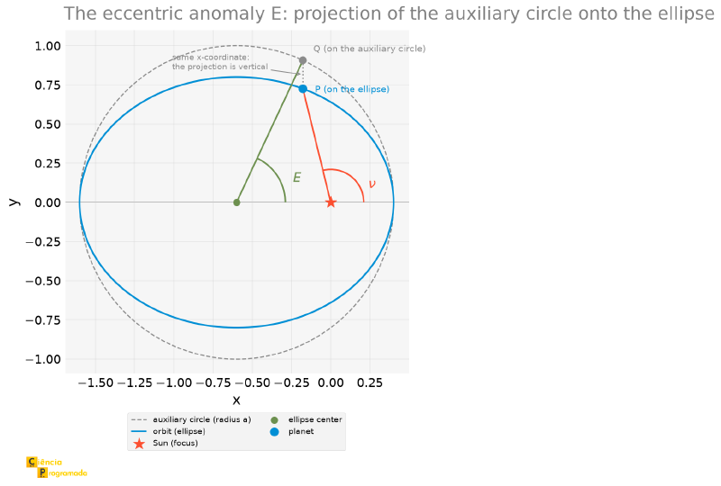
Draw, around the ellipse, the auxiliary circle: the circle of radius \(a\) (the semi-major axis) centered at the center of the ellipse. Now, given a point \(P\) of the planet on the ellipse, go up vertically until you meet the circle, at a point \(Q\).
The eccentric anomaly is the angle of point \(Q\) measured from the center of the ellipse (not from the focus), in the direction of the perihelion.
The ellipse is literally a circle flattened vertically by a factor \(b/a = \sqrt{1-e^2}\). So, if \(Q = (a\cos E,\ a\sin E)\) on the circle, the corresponding point \(P\) on the ellipse has the same abscissa and a shrunken ordinate:
$$x_{\text{center}} = a\cos E, \qquad y = a\sqrt{1-e^2}\sin E$$Since the Sun is at the focus, not at the center, we shift the origin by \(ae\) to the left, and out comes the \(x = a(\cos E - e)\) that we use in the code.
The next figure assembles this construction on an orbit of moderate eccentricity (\(e = 0.6\), chosen so the drawing stays legible): the dashed auxiliary circle, the vertical projection from \(Q\) to \(P\), and the two angles marked at their respective vertices (\(E\) at the center, \(\nu\) at the focus).
The celestial mechanics literature uses three different angles to say “where the body is in the orbit”, and swapping them is a classic mistake:
| Angle | Measured from | Used for |
|---|---|---|
| Mean, \(M\) | None (not a geometric angle) | Grows linearly with time; it is what is computed directly from the date |
| Eccentric, \(E\) | center of the ellipse | Mathematical bridge between \(M\) and the position; it is the unknown of Kepler’s equation |
| True, \(\nu\) | focus (the Sun) | It is the angle an observer on the Sun would actually see |
The mean anomaly is the strangest of the three: it does not correspond to any angle in the drawing. It is a useful fiction: the angle the body would have if it traveled around a circle at constant speed, in the same period. The whole difficulty of the problem is that nature hands us \(M\) (proportional to time) and we want \(\nu\) (the real position), and the only path between the two goes through \(E\), via the transcendental equation that has no closed form.
With that in place, the Cartesian position of the comet from \(E\) (with the Sun at the origin, semi-major axis \(a\) normalized and eccentricity \(e\)) is \(x = a(\cos E - e)\), \(y = a\sqrt{1-e^2}\sin E\). The next plot shows two panels side by side. On the left, Kepler’s equation itself as a root-finding problem, with the curve \(g(E) = E - e\sin(E)\) crossing the horizontal line \(y=M\). On the right, what that means physically: the elliptical orbit, the Sun at one of the foci, and the comet at the position corresponding to the \(E\) found.
import matplotlib.pyplot as plt
import numpy as np
from scipy import optimize


def kepler_residual(E, M, ecc):
    return E - ecc * np.sin(E) - M


def kepler_residual_prime(E, M, ecc):
    return 1 - ecc * np.cos(E)


ecc = 0.967  # eccentricity of Halley's Comet
M_val = 1.0
E_sol = optimize.newton(
    kepler_residual, x0=M_val, fprime=kepler_residual_prime, args=(M_val, ecc)
)

a_orbit = 1.0  # normalized semi-major axis

E_range = np.linspace(0, 2 * np.pi, 400)
g_E = E_range - ecc * np.sin(E_range)

fig, (ax1, ax2) = plt.subplots(1, 2, figsize=(13, 6))

# left panel: Kepler's equation as a root-finding problem
ax1.plot(E_range, g_E, color="C0", label=r"$g(E) = E - e\sin(E)$")
ax1.axhline(M_val, color="C1", linestyle="--", label=f"M = {M_val}")
ax1.scatter([E_sol], [M_val], color="C2", zorder=3, s=80, label=f"E ≈ {E_sol:.3f} rad")
ax1.set_xlabel("E (rad)")
ax1.set_ylabel("g(E)")
ax1.set_title("Kepler's equation as a root-finding problem")
ax1.legend()

# right panel: the orbit
E_orbit = np.linspace(0, 2 * np.pi, 400)
x_orbit = a_orbit * (np.cos(E_orbit) - ecc)
y_orbit = a_orbit * np.sqrt(1 - ecc**2) * np.sin(E_orbit)
x_planet = a_orbit * (np.cos(E_sol) - ecc)
y_planet = a_orbit * np.sqrt(1 - ecc**2) * np.sin(E_sol)

ax2.plot(x_orbit, y_orbit, color="C0")
ax2.scatter([0], [0], color="C1", s=200, marker="*", zorder=3, label="Sun (focus)")
ax2.scatter([x_planet], [y_planet], color="C2", s=100, zorder=3, label="comet")
ax2.plot([0, x_planet], [0, y_planet], color="gray", linestyle=":", linewidth=1)
ax2.set_aspect("equal")
ax2.set_xlabel("x")
ax2.set_ylabel("y")
ax2.set_title(f"Elliptical orbit (e = {ecc})")
ax2.legend()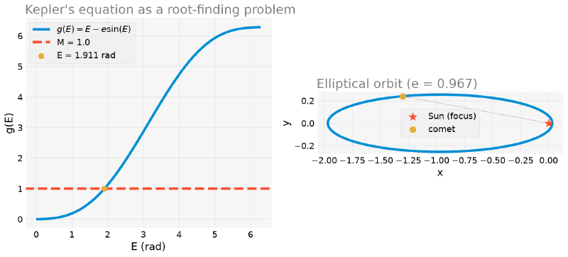
Kepler’s Second Law, Finally Visible #
So far, we used the elliptical orbit only as a geometric shape, to locate a single point on it. The other half of what Kepler discovered is still missing. The shape of the orbit differs from a circle, and the speed of the comet along it also varies, in a specific way:
The segment joining the Sun to a planet (or comet) sweeps out equal areas in equal intervals of time. Direct consequence: the body moves faster near the perihelion (the point closest to the Sun) and slower near the aphelion (the farthest point).
So far, we solved Kepler’s equation for a single instant. But the mean anomaly \(M\) was defined, by construction, to grow linearly with time; that is exactly why it is easy to compute from any date. This means that sampling \(M\) in equal steps is equivalent to sampling time in equal steps. By solving Kepler’s equation for several equally spaced \(M\) along a complete orbit, we obtain the positions of the comet at equal time intervals, and the second law becomes visible: the points should cluster near the perihelion and be spread out near the aphelion.
import matplotlib.pyplot as plt
import numpy as np
from scipy import optimize


def kepler_residual(E, M, ecc):
    return E - ecc * np.sin(E) - M


def kepler_residual_prime(E, M, ecc):
    return 1 - ecc * np.cos(E)


ecc = 0.967  # eccentricity of Halley's Comet
a_orbit = 1.0  # normalized semi-major axis

E_orbit = np.linspace(0, 2 * np.pi, 400)
x_orbit = a_orbit * (np.cos(E_orbit) - ecc)
y_orbit = a_orbit * np.sqrt(1 - ecc**2) * np.sin(E_orbit)


def orbit_positions(M_samples, ecc):
    E_samples = np.array([
        optimize.newton(kepler_residual, x0=M_i, fprime=kepler_residual_prime, args=(M_i, ecc))
        for M_i in M_samples
    ])
    x = a_orbit * (np.cos(E_samples) - ecc)
    y = a_orbit * np.sqrt(1 - ecc**2) * np.sin(E_samples)
    return x, y


n_points = 16
M_samples = np.linspace(0, 2 * np.pi, n_points, endpoint=False)
x_samples, y_samples = orbit_positions(M_samples, ecc)

fig, ax = plt.subplots(figsize=(7, 7.5))
ax.plot(x_orbit, y_orbit, color="C0", zorder=1)
ax.scatter([0], [0], color="C1", s=200, marker="*", zorder=3, label="Sun (focus)")
ax.scatter(x_samples, y_samples, color="C2", s=40, zorder=3, label="positions (equal Δt)")
for i in range(n_points):
    ax.plot([0, x_samples[i]], [0, y_samples[i]], color="gray", linewidth=0.7, zorder=0)
ax.set_aspect("equal")
ax.set_xlabel("x")
ax.set_ylabel("y")
ax.set_title("Kepler's second law: denser points near perihelion")
ax.legend(loc="upper center", bbox_to_anchor=(0.5, -0.12), ncol=2)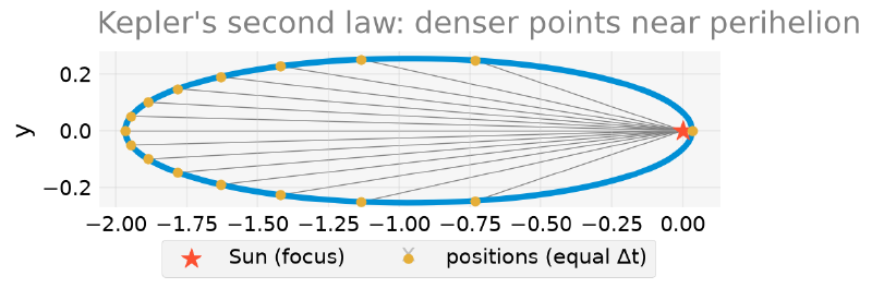
Visually, we can already notice the clustering near the perihelion (the region of the ellipse close to the Sun, on the right of the plot).
But this figure shows the radii, and the law speaks of areas. So it is worth drawing the actual areas: three sectors corresponding to the same time interval (one tenth of the period, each), taken in very different regions of the orbit.
import numpy as np
from scipy import optimize


def kepler_residual(E, M, ecc):
    return E - ecc * np.sin(E) - M


def kepler_residual_prime(E, M, ecc):
    return 1 - ecc * np.cos(E)


ecc = 0.967  # eccentricity of Halley's Comet
a_orbit = 1.0  # normalized semi-major axis


def orbit_positions(M_samples, ecc):
    E_samples = np.array([
        optimize.newton(kepler_residual, x0=M_i, fprime=kepler_residual_prime, args=(M_i, ecc))
        for M_i in M_samples
    ])
    x = a_orbit * (np.cos(E_samples) - ecc)
    y = a_orbit * np.sqrt(1 - ecc**2) * np.sin(E_samples)
    return x, y


delta_M = 2 * np.pi / 10  # one tenth of the period
sectors = {"near perihelion": 0.0,
           "midway": 2 * np.pi * 0.20,
           "near aphelion": 2 * np.pi * 0.45}

for label, M0 in sectors.items():
    M_sector = np.linspace(M0, M0 + delta_M, 300)
    xs_s, ys_s = orbit_positions(M_sector, ecc)
    xs = np.concatenate(([0.0], xs_s))   # closes the polygon at the Sun
    ys = np.concatenate(([0.0], ys_s))
    area = 0.5 * abs(np.dot(xs, np.roll(ys, -1)) - np.dot(ys, np.roll(xs, -1)))
    print(f"{label:>20}: area = {area:.5f}")
near perihelion: area = 0.08002
midway: area = 0.08004
near aphelion: area = 0.08004Equal up to the fourth decimal place. And the most impressive part is the contrast between the shapes:
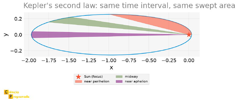
Near the perihelion, the comet travels a short arc but the distance to the Sun is small, so the sector is fat and low. Near the aphelion, it barely moves, but the radius is huge, so the sector becomes a long, very thin sliver. The two effects compensate each other exactly, and that is what the second law states.
Measuring these areas with few samples, however, holds a catch.
Approximating the area of each slice by a triangle with a vertex at the Sun (\(\text{area} = \frac{1}{2}|x_i y_{i+1} - x_{i+1} y_i|\), with the Sun at the origin) and comparing the 16 slices of the figure above, the variation among them reaches \(\mathbf{104\%}\). It looks like the second law fails. It does not: near the perihelion, where the comet changes direction fastest, the straight segment joining two consecutive positions “cuts the corner” relative to the real curved arc, underestimating the area swept there. As we increase the number of samples (each slice now covers a shorter arc of time, and the triangle approximates the curved sector better), the approximation error shrinks and the law is confirmed in practice:
import numpy as np
from scipy import optimize


def kepler_residual(E, M, ecc):
    return E - ecc * np.sin(E) - M


def kepler_residual_prime(E, M, ecc):
    return 1 - ecc * np.cos(E)


ecc = 0.967  # eccentricity of Halley's Comet
a_orbit = 1.0  # normalized semi-major axis


def orbit_positions(M_samples, ecc):
    E_samples = np.array([
        optimize.newton(kepler_residual, x0=M_i, fprime=kepler_residual_prime, args=(M_i, ecc))
        for M_i in M_samples
    ])
    x = a_orbit * (np.cos(E_samples) - ecc)
    y = a_orbit * np.sqrt(1 - ecc**2) * np.sin(E_samples)
    return x, y


def slice_areas(x, y):
    x_next, y_next = np.roll(x, -1), np.roll(y, -1)
    return 0.5 * np.abs(x * y_next - x_next * y)


for n_test in [16, 100, 1000, 5000]:
    M_test = np.linspace(0, 2 * np.pi, n_test, endpoint=False)
    x_test, y_test = orbit_positions(M_test, ecc)
    areas_test = slice_areas(x_test, y_test)
    rel_var = (areas_test.max() - areas_test.min()) / areas_test.mean()
    print(f"n = {n_test:5d} points: relative variation of areas = {rel_var:.2%}")
n = 16 points: relative variation of areas = 104.29%
n = 100 points: relative variation of areas = 69.60%
n = 1000 points: relative variation of areas = 12.45%
n = 5000 points: relative variation of areas = 0.72%With 5000 samples, the slices are already practically equal; the law was right all along, it just needed enough resolution to show up in the numbers.
Near the Extreme Perihelion: Newton Slows Down #
Newton with a derivative converges quickly for moderate eccentricities, but convergence worsens as \(e \to 1\): increasingly elongated orbits, the regime of long-period comets. Solving the same Kepler equation for \(M=1\) rad, varying only the eccentricity, and counting how many iterations Newton needs until the residual falls below \(10^{-12}\):
import matplotlib.pyplot as plt
import numpy as np


def kepler_residual(E, M, ecc):
    return E - ecc * np.sin(E) - M


def kepler_residual_prime(E, M, ecc):
    return 1 - ecc * np.cos(E)


def newton_count_iterations(f, fp, x0, args, tol=1e-12, max_iter=100):
    x = x0
    for i in range(1, max_iter + 1):
        fx = f(x, *args)
        if abs(fx) < tol:
            return i
        x = x - fx / fp(x, *args)
    return max_iter  # did not converge within this limit


ecc = 0.967  # eccentricity of Halley's Comet
M_val = 1.0

eccs = np.linspace(0.1, 0.99, 40)
iterations = [
    newton_count_iterations(kepler_residual, kepler_residual_prime, M_val, args=(M_val, e_i))
    for e_i in eccs
]

halley_iter = newton_count_iterations(
    kepler_residual, kepler_residual_prime, M_val, args=(M_val, ecc)
)
print(f"Halley (e={ecc}): {halley_iter} iterations")

fig, ax = plt.subplots(figsize=(8, 5))
ax.plot(eccs, iterations, "o-", color="C0")
ax.scatter([ecc], [halley_iter], color="C1", zorder=3, s=80, label=f"Halley (e={ecc})")
ax.legend()
ax.set_xlabel("eccentricity (e)")
ax.set_ylabel("iterations to converge")
ax.set_title("Newton slows down near almost parabolic orbits")
Halley (e=0.967): 7 iterations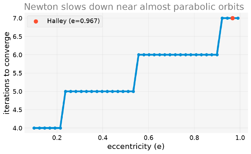
The relationship is not smooth: the number of iterations rises in steps (from 4 to 5 at \(e \approx 0.23\), from 5 to 6 at \(e \approx 0.55\), from 6 to 7 at \(e \approx 0.92\)), because it is an integer count of steps until crossing the tolerance, not a continuous quantity. Even so, the trend is clear: Halley’s Comet, with \(e \approx 0.967\), is already on the slowest plateau observed in this range. Even more elongated orbits (very long-period comets, with \(e\) above \(0.99\)) would require even more iterations, or an initial guess better than \(M\) to speed up convergence.
Why Kepler Needed Mars, and Not Earth #
The same code answers a historical question that usually goes unnoticed: why did Kepler spend years analyzing data on Mars, and not on the planet right under his feet?
import numpy as np
from scipy import optimize


def kepler_residual(E, M, ecc):
    return E - ecc * np.sin(E) - M


def kepler_residual_prime(E, M, ecc):
    return 1 - ecc * np.cos(E)


def newton_count_iterations(f, fp, x0, args, tol=1e-12, max_iter=100):
    x = x0
    for i in range(1, max_iter + 1):
        fx = f(x, *args)
        if abs(fx) < tol:
            return i
        x = x - fx / fp(x, *args)
    return max_iter  # did not converge within this limit


for name, e_i in [("Earth", 0.0167), ("Mars", 0.0934), ("Halley", 0.967)]:
    E_i = optimize.newton(kepler_residual, x0=1.0, fprime=kepler_residual_prime,
                          args=(1.0, e_i))
    iterations_i = newton_count_iterations(kepler_residual, kepler_residual_prime,
                                           1.0, args=(1.0, e_i))
    print(f"{name:>7}  e={e_i:.4f}  b/a={np.sqrt(1 - e_i**2):.4f}  "
          f"E={E_i:.4f} rad  ({iterations_i} iterations)")
Earth e=0.0167 b/a=0.9999 E=1.0142 rad (3 iterations)
Mars e=0.0934 b/a=0.9956 E=1.0825 rad (4 iterations)
Halley e=0.9670 b/a=0.2548 E=1.9114 rad (7 iterations)Earth’s orbit has \(b/a = 0.9999\): it differs from a perfect circle by 0.014%. This flattening is on the order of the error of the best sixteenth century observations (0.5’ to 1’ in those of Tycho Brahe): drawn on paper, Earth’s orbit is a circle. Mars, with \(e = 0.0934\), is still almost circular (\(b/a = 0.9956\)), but it has a decisive advantage: since the Sun is at the focus, not at the center, the Sun-Mars distance varies by \(\pm 9.3\%\) over the Martian year, against \(\pm 1.7\%\) for Earth.
It was this variation, not the flattening, that showed up in Tycho Brahe’s data. Kepler spent most of a decade in what he called the “war on Mars” precisely because Mars was the planet with good data whose orbit departed enough from a circle to give the ellipse away. With Earth, or with Venus (\(e = 0.007\)), the discovery simply would not be in the numbers.
Notice also the iterations column: 3 for Earth, 7 for Halley. It is the same trend that the next section measures in detail.
Projectile with Air Resistance #
The second problem leaves celestial mechanics and returns to Earth: a projectile launched with initial speed \(v_0\) and angle \(\theta\), under drag proportional to the speed (\(F_{\text{drag}} = -kmv\)). The height as a function of time has an exponential term:
$$ y(t) = \frac{v_{0y} + g/k}{k}\left(1 - e^{-kt}\right) - \frac{gt}{k} $$Finding the flight time, the instant when the height returns to zero, means solving a transcendental equation in \(t\).
Drag proportional to the speed (\(F \propto v\), called Stokes drag) holds at low Reynolds number: microscopic droplets, spheres falling in a viscous liquid. A projectile at \(30\) m/s in air is firmly in the opposite regime, where drag is proportional to the square of the speed (\(F \propto v^2\)).
So why use the linear one? Because it is the only one that still has a
closed-form trajectory, and that is precisely what enables the comparison
in this article: one exact analytic curve against another, with the only
unknown (the flight time) falling to a brentq. With quadratic drag there
is no closed formula left for the 2D trajectory.
The quadratic case, the physically correct one, is solved in Differential Equations with SciPy, and there the tool changes: instead of a transcendental equation for the flight time, we integrate the differential equation in time. Read the numbers below, therefore, as “the qualitative effect of drag”, not as real ballistics.
And there is a trap before that, exactly the kind the previous article taught us to look for: the height is zero at two instants, at launch and at landing. \(t = 0\) is a legitimate root of the equation, and without care it is the one the solver finds. That is why the bracket used next starts at \(0.1\) s, not at zero: it deliberately excludes the trivial root.
Technically, it is possible to isolate \(t\) in this equation using the Lambert W function, the inverse of \(f(w) = we^w\). But this function rarely shows up in introductory courses, and in practice the standard route is numerical anyway, which makes this a legitimate example of “no useful closed form”, even when a formal solution exists.
Example 2: flight time with air resistance
Statement: A projectile is launched at \(v_0 = 30\) m/s, at an angle of \(45°\), with drag coefficient \(k = 0.2\) s⁻¹. How long does it stay in the air?
Solution:
import numpy as np
from scipy import optimize


g = 9.81
k_drag = 0.2  # drag coefficient / mass
v0 = 30.0  # m/s
angle_deg = 45.0
v0x = v0 * np.cos(np.radians(angle_deg))
v0y = v0 * np.sin(np.radians(angle_deg))


def height(t):
    return (v0y + g / k_drag) / k_drag * (1 - np.exp(-k_drag * t)) - g * t / k_drag


flight_time = optimize.brentq(height, 0.1, 20)
print("flight time (with air resistance):", flight_time, "s")
flight time (with air resistance): 3.838446938469727 sThe next plot shows the height over time, with the root, the flight time, marked where the curve crosses zero again.
import matplotlib.pyplot as plt
import numpy as np
from scipy import optimize


g = 9.81
k_drag = 0.2  # drag coefficient / mass
v0 = 30.0  # m/s
angle_deg = 45.0
v0x = v0 * np.cos(np.radians(angle_deg))
v0y = v0 * np.sin(np.radians(angle_deg))


def height(t):
    return (v0y + g / k_drag) / k_drag * (1 - np.exp(-k_drag * t)) - g * t / k_drag


flight_time = optimize.brentq(height, 0.1, 20)

t_range = np.linspace(0, flight_time * 1.2, 300)
fig, ax = plt.subplots(figsize=(8, 5))
ax.plot(t_range, height(t_range), color="C0")
ax.axhline(0, color="gray", linewidth=1, zorder=0)
ax.scatter([flight_time], [0], color="C2", zorder=3, label="flight time")
ax.legend()
ax.set_xlabel("t (s)")
ax.set_ylabel("height (m)")
ax.set_title("Projectile with linear air resistance")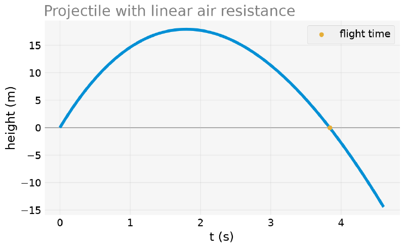
How Much Does Air Resistance Really Change the Trajectory? #
The ideal case (no drag) has a closed-form trajectory and flight time: \(t_{\text{flight}}^{\text{ideal}} = 2v_{0y}/g\). Overlaying the two complete trajectories (position \(x(t)\) against \(y(t)\), not just height against time), it becomes visible how much drag reduces the range.
import matplotlib.pyplot as plt
import numpy as np
from scipy import optimize


g = 9.81
k_drag = 0.2  # drag coefficient / mass
v0 = 30.0  # m/s
angle_deg = 45.0
v0x = v0 * np.cos(np.radians(angle_deg))
v0y = v0 * np.sin(np.radians(angle_deg))


def height(t):
    return (v0y + g / k_drag) / k_drag * (1 - np.exp(-k_drag * t)) - g * t / k_drag


flight_time = optimize.brentq(height, 0.1, 20)

ideal_flight_time = 2 * v0y / g
t_range_ideal = np.linspace(0, ideal_flight_time, 300)
x_ideal = v0x * t_range_ideal
y_ideal = v0y * t_range_ideal - 0.5 * g * t_range_ideal**2

t_range_drag = np.linspace(0, flight_time, 300)
x_drag = v0x / k_drag * (1 - np.exp(-k_drag * t_range_drag))
y_drag = height(t_range_drag)

fig, ax = plt.subplots(figsize=(9, 5))
ax.plot(x_ideal, y_ideal, color="C0", label="without air resistance (closed form)")
ax.plot(x_drag, y_drag, color="C1", label="with air resistance (numerical)")
ax.scatter([x_ideal[-1]], [0], color="C0", zorder=3)
ax.scatter([x_drag[-1]], [0], color="C1", zorder=3)
ax.axhline(0, color="gray", linewidth=1, zorder=0)
ax.set_ylim(0, y_ideal.max() * 1.4)  # room at the top so the legend does not cover the curves
ax.legend(loc="upper right")
ax.set_xlabel("x (m)")
ax.set_ylabel("y (m)")
ax.set_title("Trajectory: with × without air resistance")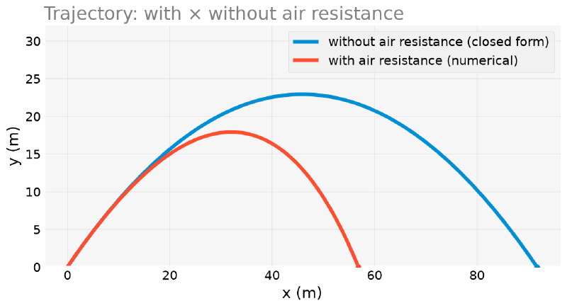
import numpy as np
from scipy import optimize


g = 9.81
k_drag = 0.2  # drag coefficient / mass
v0 = 30.0  # m/s
angle_deg = 45.0
v0x = v0 * np.cos(np.radians(angle_deg))
v0y = v0 * np.sin(np.radians(angle_deg))


def height(t):
    return (v0y + g / k_drag) / k_drag * (1 - np.exp(-k_drag * t)) - g * t / k_drag


flight_time = optimize.brentq(height, 0.1, 20)

ideal_flight_time = 2 * v0y / g
ideal_range = v0x * ideal_flight_time
drag_range = v0x / k_drag * (1 - np.exp(-k_drag * flight_time))

print(f"ideal range: {ideal_range:.1f} m (flight_time = {ideal_flight_time:.2f} s)")
print(f"range with air resistance: {drag_range:.1f} m (flight_time = {flight_time:.2f} s)")
ideal range: 91.7 m (flight_time = 4.32 s)
range with air resistance: 56.8 m (flight_time = 3.84 s)With \(k = 0.2\), drag cuts the range by about 38% (from \(91.7\) m to \(56.8\) m) and reduces the flight time by half a second. The lesson lies more in the order of magnitude of the error than in the exact number (which depends on the linear model, as warned above): ignoring air resistance produces a deviation of tens of percent, not a few. That is why the high school parabola, however elegant it may be, is of no use for any practical ballistics application, and why it is worth learning to solve the resisted case, even when it costs a numerical root instead of a formula.
How Much Does the Drag Coefficient Matter? #
k_drag = 0.2 was a single value, chosen for the example above. This
coefficient depends on the shape of the projectile, frontal area, air
density, and, crucially, mass: the \(k\) that appears in the formulas is
the ratio between the raw drag coefficient and the mass of the projectile,
\(k = b/m\), with unit s⁻¹. That is why a tennis ball and a cannonball of
the same size behave so differently: same frontal area, same \(b\), very
different masses, and therefore very different \(k\). By repeating the
same brentq over a range of \(k\) values, we can see how the range and
the flight time behave without needing any new tool.
import matplotlib.pyplot as plt
import numpy as np
from scipy import optimize


g = 9.81
k_drag = 0.2  # drag coefficient / mass
v0 = 30.0  # m/s
angle_deg = 45.0
v0x = v0 * np.cos(np.radians(angle_deg))
v0y = v0 * np.sin(np.radians(angle_deg))


def height(t):
    return (v0y + g / k_drag) / k_drag * (1 - np.exp(-k_drag * t)) - g * t / k_drag


flight_time = optimize.brentq(height, 0.1, 20)

drag_range = v0x / k_drag * (1 - np.exp(-k_drag * flight_time))


def height_with_k(t, k):
    return (v0y + g / k) / k * (1 - np.exp(-k * t)) - g * t / k


def range_with_k(k):
    flight_time_k = optimize.brentq(height_with_k, 0.1, 20, args=(k,))
    range_k = v0x / k * (1 - np.exp(-k * flight_time_k))
    return range_k, flight_time_k


k_range = np.linspace(0.02, 0.6, 40)
results = [range_with_k(k_i) for k_i in k_range]
ranges = [r[0] for r in results]
flight_times = [r[1] for r in results]

fig, (ax1, ax2) = plt.subplots(1, 2, figsize=(12, 5))
ax1.plot(k_range, ranges, color="C0")
ax1.scatter([k_drag], [drag_range], color="C2", zorder=3, label=f"k = {k_drag}")
ax1.set_xlabel("drag coefficient (k)")
ax1.set_ylabel("range (m)")
ax1.set_title("Range vs. drag")
ax1.legend()

ax2.plot(k_range, flight_times, color="C1")
ax2.scatter([k_drag], [flight_time], color="C2", zorder=3, label=f"k = {k_drag}")
ax2.set_xlabel("drag coefficient (k)")
ax2.set_ylabel("flight time (s)")
ax2.set_title("Flight time vs. drag")
ax2.legend()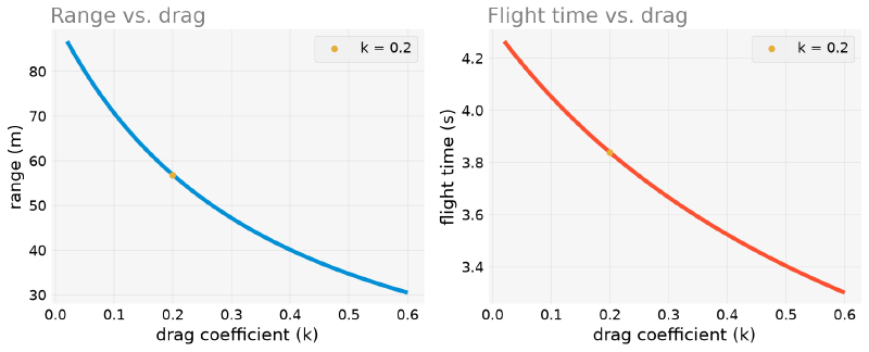
At the extremes tested, the range falls from \(86.7\) m (\(k = 0.02\), almost negligible drag) to \(30.5\) m (\(k = 0.6\), strong drag), less than a third. The drop is smooth and monotonic: there is no qualitative surprise here, unlike what happened with Kepler’s eccentricity (where steps appeared). It makes sense: more drag always means less range, with no special threshold behavior.
Summary Table #
| Problem | Equation | Method | Result |
|---|---|---|---|
| Position of Halley’s Comet | \(M = E - e\sin(E)\) | newton (with derivative) |
\(E \approx 1.911\) rad for \(M=1\), \(e \approx 0.967\) |
| Kepler’s second law | Areas of the slices between positions | newton (several samples) + numerical check |
Relative variation drops from 104% (n=16) to 0.72% (n=5000) |
| Convergence near \(e \to 1\) | Same Kepler equation | Iteration count of newton |
From 4 to 7 iterations in the range \(e \in [0.1, 0.99]\) |
| Flight time with linear drag | \(y(t) = 0\), exponential form | brentq |
\(t_{\text{flight}} \approx 3.84\) s, range \(\approx 56.8\) m (against \(91.7\) m in the ideal case without drag) |
| Sensitivity to drag | Same equation, variable \(k\) | repeated brentq |
Range from \(86.7\) m to \(30.5\) m for \(k \in [0.02, 0.6]\) |
Next Steps #
The two problems in this article came from physics (one from celestial
mechanics, the other from ballistics) and each used a single real numerical
scenario (Halley’s Comet, a launch at \(45°\)) instead of isolated
didactic examples. But physics is not the only domain where equations with
no closed form show up all the time. Chemistry and engineering have their
own, with different traps: cubics with multiple physical roots, classroom
approximations that stop holding, and implicit equations that engineers
solved by hand decades before scipy.optimize existed.
In the next article, From Chemistry to Engineering, we solve three of these real equations (the molar volume of a real gas, the pH of a weak acid, and the Colebrook friction factor), all with the same tools presented in this block.


